SAMPLE SIZE REQUIREMENTS FOR STRATIFIED RANDOM SAMPLING OF

SAMPLE SIZE REQUIREMENTS FOR STRATIFIED RANDOM SAMPLING OF AGRICULTURAL RUN OFF POLLUTANTS IN POND WATER WITH COST CONSIDERATIONS USING A BAYESIAN METHODOLOGY A. A. Bartolucci Department of Biostatistics, University of Alabama at Birmingham, Alabama 35294 -0022 USA S. Bae and K. P. Singh Department of Biostatistics, School of Public Health, University of North Texas Health Science Center at Forth Worth, Texas 76107 -2699 USA

GOAL: USING A BAYESIAN APPROACH WE WISH TO DETERMINE THE OPTIMUM SAMPLE SIZE , n, AND SAMPLE SIZE, nh , FOR SAMPLING WITHIN STRATUM, h, WHERE h=1, 2, . . . L AND n=n 1+n 2+. . . . +n. L. THE STRATA ARE BASICALLY DEPTH LEVELS IN A POND. SAMPLING IS TO DETERMINE THE AMOUNT OF POLLUTION IN THE POND.

Three Approaches 1. Pre Specified Margin of Error (PMOE) 2. Pre Specified Fixed Cost 3. Correlation Structure Among the Strata

TRADITIONAL SETUP N=Total number of population units in the target population. For L strata, h=1, . . . . L , . n = total number of sampling units in the target sample. n = n 1 +n 2 +. . . n. L =

Weight of stratum h, Wh =Nh / N. The mean, μ, of the population of n units: Estimate uh by : where xhi =ith observation in stratum h.

An unbiased estimator of μ is : Let Nh / N = nh / n in all strata, then

Variance: Var(mst) = Estimate the stratum variance, σ2 h , by It can be shown that for large N,

Optimum n: Using Prespecified Margin of Error PMOE Let d= pre specified margin of error, i. e. d=|mst -μ| that can be tolerated and a small probability, α, of exceeding that error. i. e. P( |mst -μ| d) = α. Then by Cochran an optimum n is:

For N , Thus the optimal nh for each h is: For our example we let d=0. 2 and α =0. 10.

Optimum n: Using Prespecified Fixed Cost where ch is the cost per population unit in the hth stratum and c 0 is the fixed overhead cost. Thus the optimum n is:

As above, the optimum nh per stratum is: Our examples will reflect both conditions of prespecified margin of error and prespecified fixed cost.

Correlation Among the Depth Strata Let ρc = the average correlation among the depth strata, i. e. average of all possible pairwise correlations. Let ns = number of strata. ns=L. Let nh = the number to be sampled in each of the L strata or nh =stratum size. Thus:

Bayesian Considerations Derivation of the posterior variance using the Bayesian approach to the solution of the Behren’s Fisher problem for inference on mean (μ) and variance (σ) of the normal distribution when both paramters are unknown. Likelihood function for n observations: υ=n-1, nm=x 1 + x 2 +. . . xn , υs 2 = (x 1 -m)2 +(x 2 -m)2+. . . + (xn-m)2.

Consider the t-density: φ(x; s 2) = s-1[υ1/2 Beta(υ/2, 1/2)]-1(1+υ-1(x/s)2)(υ+1)/2 where The prior for the mean, μ, is: normal for υo .

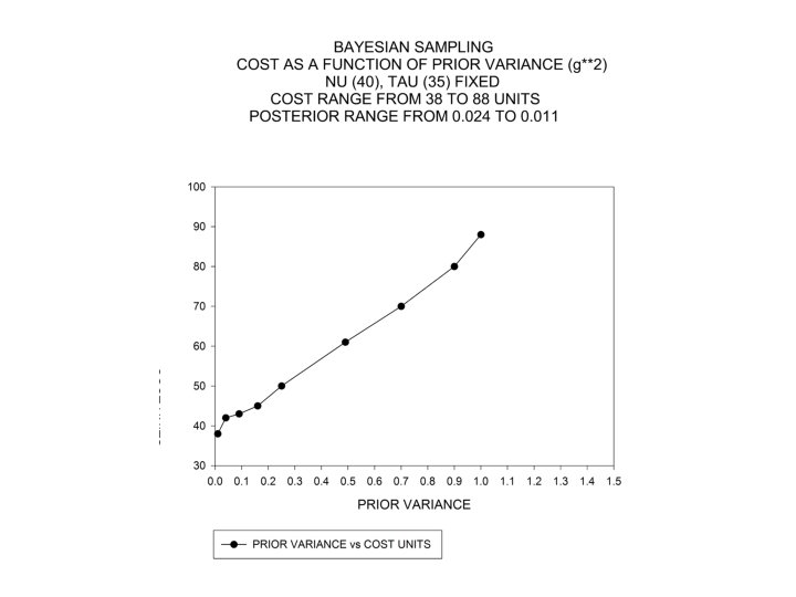
Prior: p( 2) g 2/ 2 Let B=υ+τ. The posterior variance is: ε 2 = (υs 2+τg 2)/B. Thus substitute ε 2 h for s 2 h in the above computations of n and nh.

Example: Estimate the average phosphorous concentration (μg/100 ml) in Pond water. The phosphorous concentration of a 100 -ml aliquot from each 1 -Liter sample will be measured. N=total number of 100 -ml water samples in the pond. Nh =number of aliquots in stratum h. There are five strata of depth levels, h=1, 2, . . 5

Table 1. Data for stratified random sampling to estimate samples per strata (PMOE) Classical Approach (υ =1, τ =0, g =1) s 2(mst) = 0. 0140, Cost=74 (For cost per strata please see next slide) Strata Nh Wh nh mh s 2 h 1 4. 25 M 3 0. 266 10 1. 67 0. 4376 2 3. 96 0. 248 9 2. 83 0. 4228 3 3. 23 0. 202 8 3. 59 0. 5339 4 2. 85 0. 178 9 4. 23 0. 7222 5 1. 70 0. 106 7 5. 31 1. 3920 Total 15. 99 1. 000 43 - -

The unit cost to sample each depth level is: Level (h) Cost 1 1 2 1 3 2 4 2 5 3 The assumption being that the cost is higher at greater depths.

Table 2. Bayesian Results (PMOE) (υ, τ, g) n 1 n 2 n 3 n 4 n 5 35, 1, 0. 5 9 9 8 8 7 35, 2, 0. 5 9 8 8 8 20, 1, 1. 0 9 8 8 40, 35, 0. 2 5 5 40, 35, 0. 5 7 7 Total s 2(mst) Cost 41 0. 0140 71 7 40 0. 0141 70 8 6 39 0. 0138 67 4 4 4 22 0. 0143 38 6 6 4 30 0. 0195 42

Table 3. Pre specified fixed cost (Bayesian results in bottom row) C-c 0 υ τ g n n 1 n 2 n 3 n 4 n 5 50 - - - 31 7 7 6 6 5+ 50 40 35 0. 12 31 7 7 6 6 5

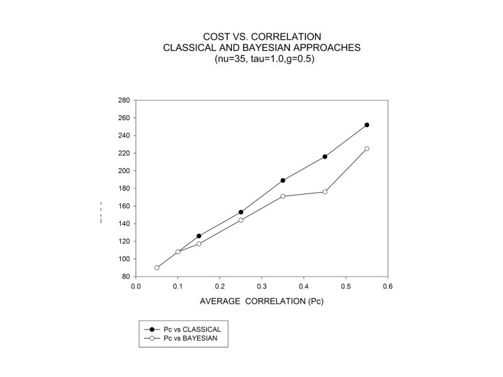
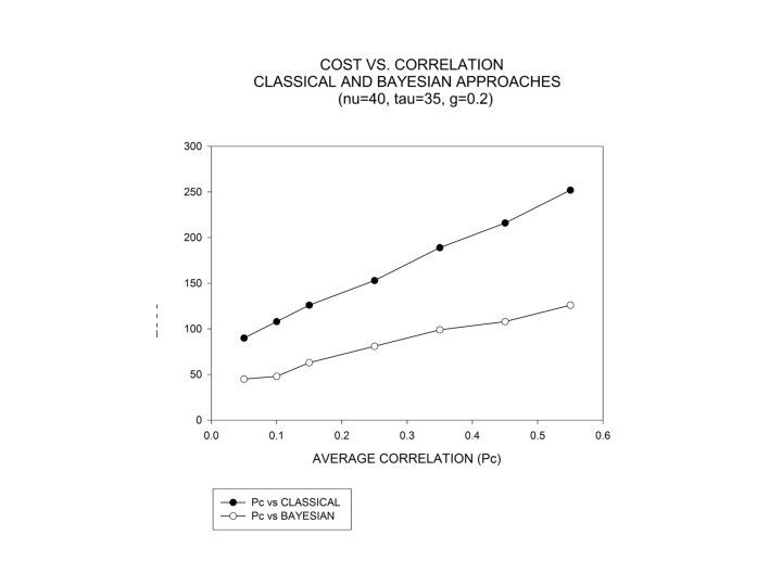
Table 4. Example Using the Correlation Structure, ρc. prior (υ, τ, g) Classical (35, 1, 0. 5) Cost nh (20, 1, 0. 1) (40, 35, . 2) Cost nh Cost ρc nh 0. 05 10 90 05 45 0. 10 12 108 11 108 06 48 0. 15 14 126 13 117 07 63 0. 25 17 153 16 144 09 81 0. 35 21 189 20 180 19 171 11 99 0. 45 24 216 23 207 22 176 12 108 0. 55 28 252 26 234 25 225 14 126

Conclusions: Compared to the classical sampling analysis for the pre specified margin of error approach as well as the correlational approach, the Bayesian analysis resulted in: 1. Reduction in required number of samples thus lowering the cost , especially when realistic (empirical) prior hyperparameters are utilized. 2. No serious adverse impact on standard error of the estimates of the mean concentration.

- There were no real differences between classical and Bayesian approaches in the pre specified fixed cost analysis - Given current computational tools the Bayesian calculations proved to be fairly straight forward. - Given the current availability of databases, future Bayesian approaches to environmental sampling should be given serious consideration.