Quantitative Modelling of the Shifts and Splitting in

Quantitative Modelling of the Shifts and Splitting in the Infrared Spectra of SF 6 in an Ar Matrix ‡ Tao Peng and Robert J. Le Roy Guelph-Waterloo Centre for Graduate Work in Chemistry and Biochemistry, University of Waterloo 60 th International Symposium on Molecular Spectroscopy, June 22, 2005 ‡ Research supported by the Natural Sciences and Engineering Research Council of Canada

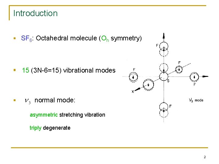
Introduction § SF 6: Octahedral molecule (Oh symmetry) § 15 (3 N-6=15) vibrational modes § normal mode: asymmetric stretching vibration triply degenerate 2

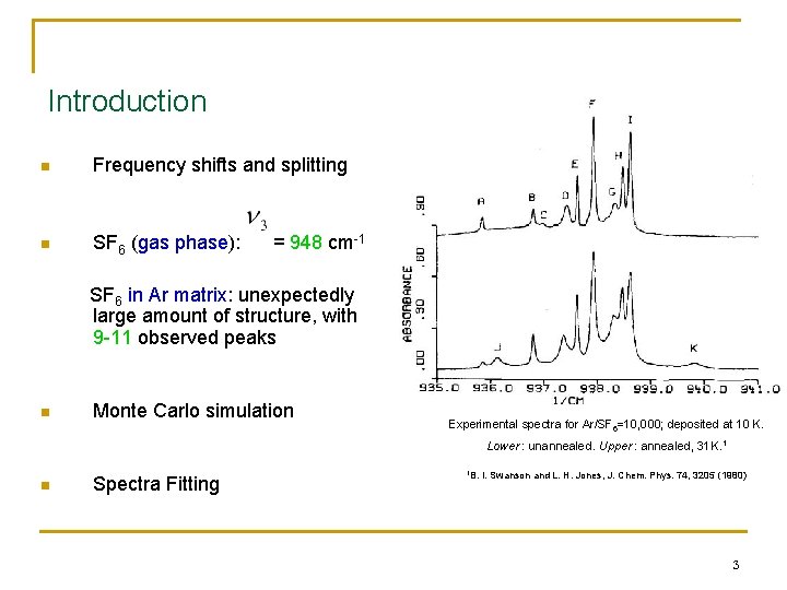
Introduction n Frequency shifts and splitting n SF 6 (gas phase): = 948 cm-1 SF 6 in Ar matrix: unexpectedly large amount of structure, with 9 -11 observed peaks n Monte Carlo simulation Experimental spectra for Ar/SF 6=10, 000; deposited at 10 K. Lower : unannealed. Upper : annealed, 31 K. 1 n Spectra Fitting 1 B. I. Swanson and L. H. Jones, J. Chem. Phys. 74, 3205 (1980) 3

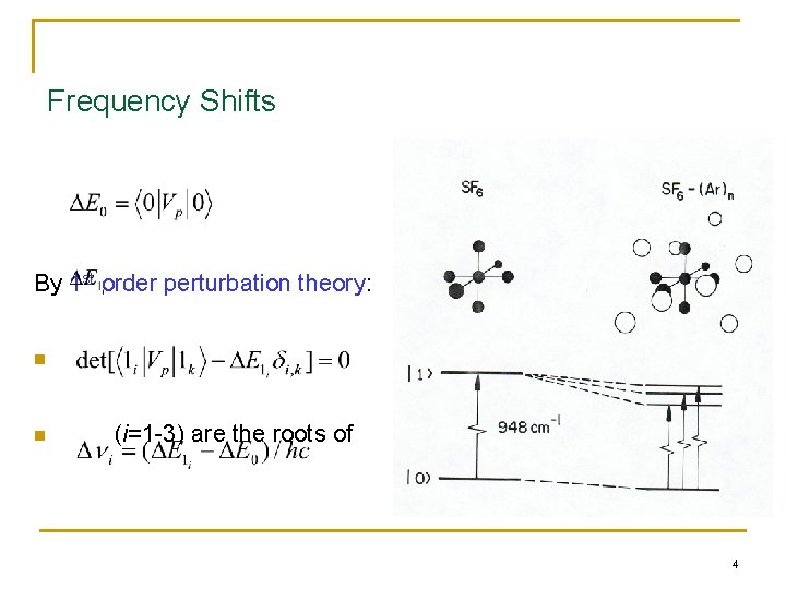
Frequency Shifts By 1 st order perturbation theory: n n (i=1 -3) are the roots of 4

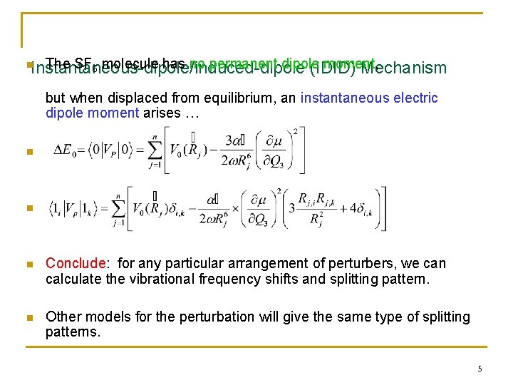
The SF 6 molecule has no permanent dipole moment, Instantaneous-dipole/induced-dipole (IDID) Mechanism n but when displaced from equilibrium, an instantaneous electric dipole moment arises … n n n Conclude: for any particular arrangement of perturbers, we can calculate the vibrational frequency shifts and splitting pattern. n Other models for the perturbation will give the same type of splitting patterns. 5

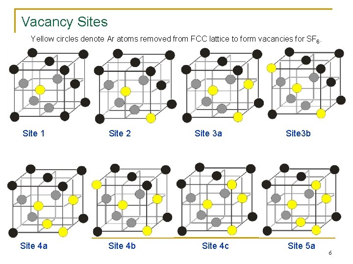
Vacancy Sites Yellow circles denote Ar atoms removed from FCC lattice to form vacancies for SF 6. Site 1 Site 2 Site 4 a Site 4 b Site 3 a Site 4 c Site 3 b Site 5 a 6

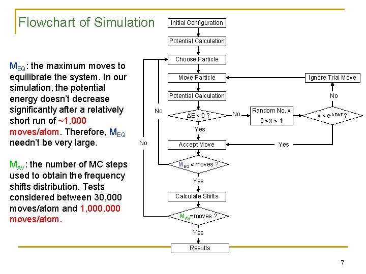
Flowchart of Simulation Initial Configuration Potential Calculation MEQ: the maximum moves to equilibrate the system. In our simulation, the potential energy doesn’t decrease significantly after a relatively short run of ~1, 000 moves/atom. Therefore, MEQ needn’t be very large. MAV: the number of MC steps used to obtain the frequency shifts distribution. Tests considered between 30, 000 moves/atom and 1, 000 moves/atom. Choose Particle No Move Particle Ignore Trial Move Potential Calculation No ΔE ≤ 0 ? No Random No. x 0≤x≤ 1 x ≤ e-ΔE/k. T ? Yes No Accept Move Yes MEQ ≤ moves ? Yes Calculate Shifts MAV=moves ? Yes Results 7

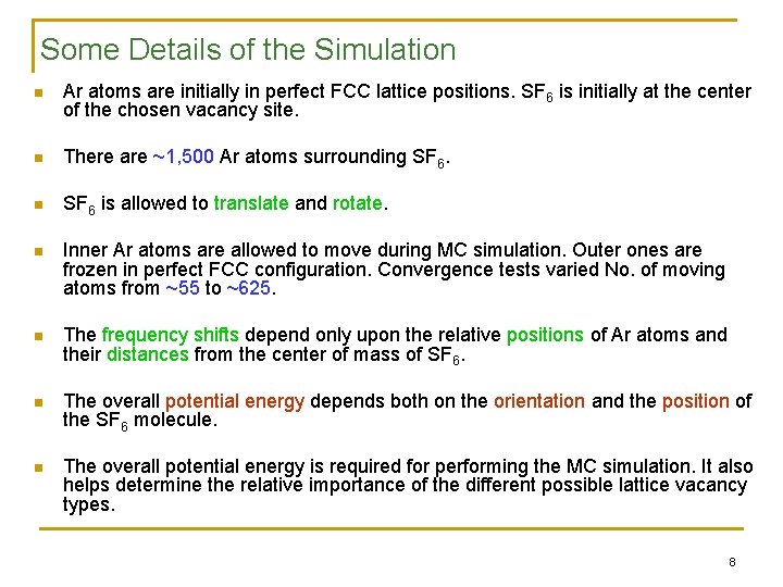
Some Details of the Simulation n Ar atoms are initially in perfect FCC lattice positions. SF 6 is initially at the center of the chosen vacancy site. n There are ~1, 500 Ar atoms surrounding SF 6. n SF 6 is allowed to translate and rotate. n Inner Ar atoms are allowed to move during MC simulation. Outer ones are frozen in perfect FCC configuration. Convergence tests varied No. of moving atoms from ~55 to ~625. n The frequency shifts depend only upon the relative positions of Ar atoms and their distances from the center of mass of SF 6. n The overall potential energy depends both on the orientation and the position of the SF 6 molecule. n The overall potential energy is required for performing the MC simulation. It also helps determine the relative importance of the different possible lattice vacancy types. 8

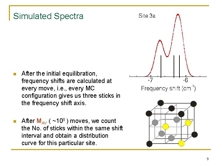
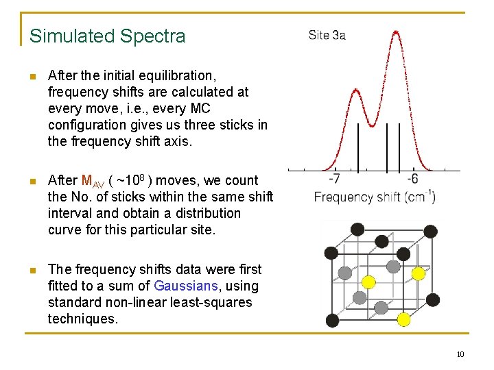
Simulated Spectra n After the initial equilibration, frequency shifts are calculated at every move, i. e. , every MC configuration gives us three sticks in the frequency shift axis. n After MAV ( ~108 ) moves, we count the No. of sticks within the same shift interval and obtain a distribution curve for this particular site. 9

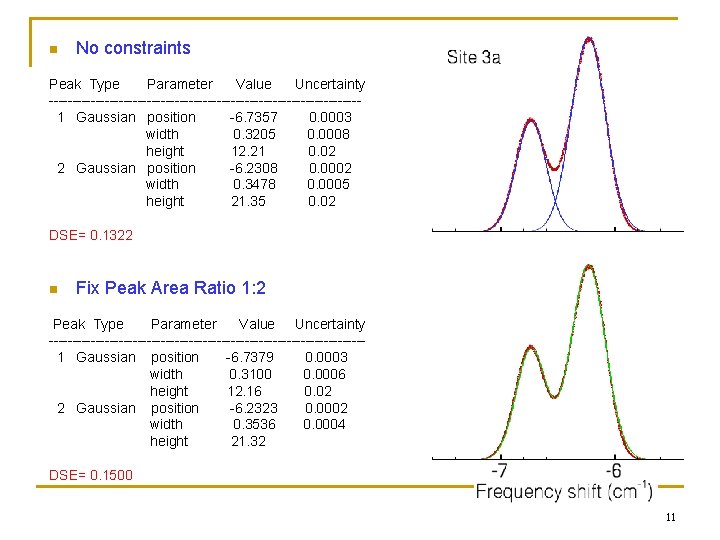
Simulated Spectra n After the initial equilibration, frequency shifts are calculated at every move, i. e. , every MC configuration gives us three sticks in the frequency shift axis. n After MAV ( ~108 ) moves, we count the No. of sticks within the same shift interval and obtain a distribution curve for this particular site. n The frequency shifts data were first fitted to a sum of Gaussians, using standard non-linear least-squares techniques. 10

n No constraints Peak Type Parameter Value Uncertainty ---------------------------------1 Gaussian position -6. 7357 0. 0003 width 0. 3205 0. 0008 height 12. 21 0. 02 2 Gaussian position -6. 2308 0. 0002 width 0. 3478 0. 0005 height 21. 35 0. 02 DSE= 0. 1322 n Fix Peak Area Ratio 1: 2 Peak Type Parameter Value Uncertainty ----------------------------------1 Gaussian position -6. 7379 0. 0003 width 0. 3100 0. 0006 height 12. 16 0. 02 2 Gaussian position -6. 2323 0. 0002 width 0. 3536 0. 0004 height 21. 32 DSE= 0. 1500 11

12

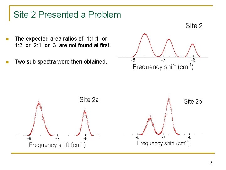
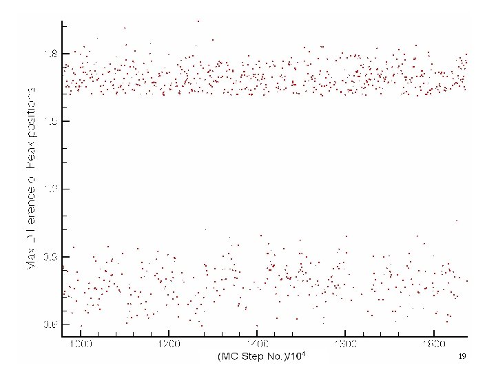
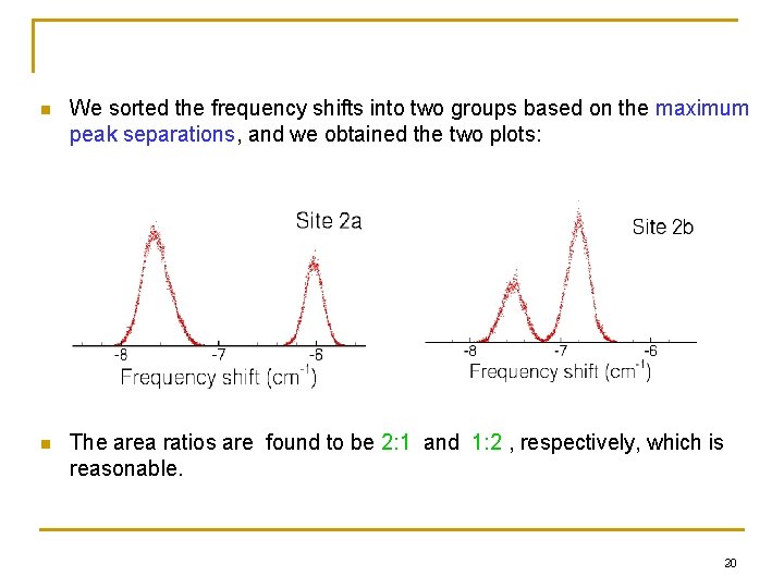
Site 2 Presented a Problem n The expected area ratios of 1: 1: 1 or 1: 2 or 2: 1 or 3 are not found at first. n Two sub spectra were then obtained. 13

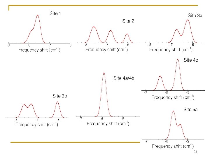
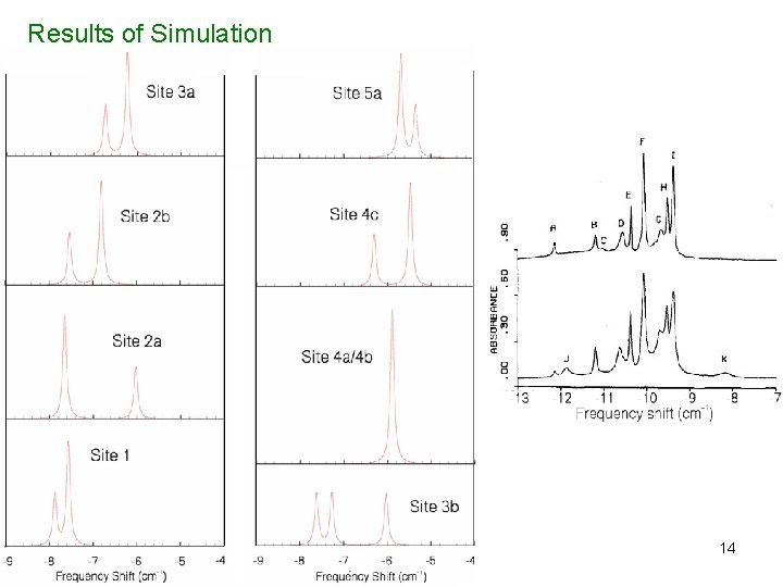
Results of Simulation 14

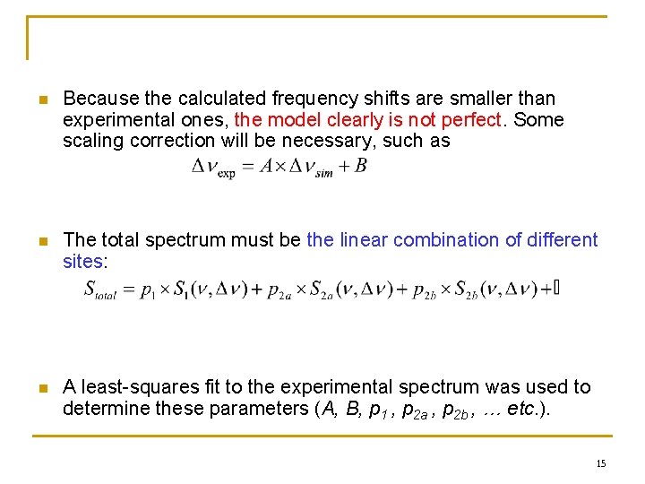
n Because the calculated frequency shifts are smaller than experimental ones, the model clearly is not perfect. Some scaling correction will be necessary, such as n The total spectrum must be the linear combination of different sites: n A least-squares fit to the experimental spectrum was used to determine these parameters (A, B, p 1 , p 2 a , p 2 b , … etc. ). 15

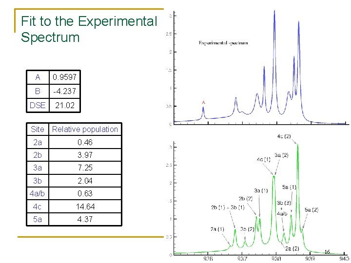
Fit to the Experimental Spectrum A 0. 9597 B -4. 237 DSE 21. 02 Site Relative population 2 a 0. 46 2 b 3. 97 3 a 7. 25 3 b 2. 04 4 a/b 0. 63 4 c 14. 64 5 a 4. 37 16

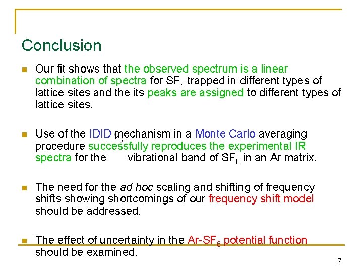
Conclusion n Our fit shows that the observed spectrum is a linear combination of spectra for SF 6 trapped in different types of lattice sites and the its peaks are assigned to different types of lattice sites. n Use of the IDID mechanism in a Monte Carlo averaging procedure successfully reproduces the experimental IR spectra for the vibrational band of SF 6 in an Ar matrix. n The need for the ad hoc scaling and shifting of frequency shifts showing shortcomings of our frequency shift model should be addressed. n The effect of uncertainty in the Ar-SF 6 potential function should be examined. 17

Thank You! 18

19

n We sorted the frequency shifts into two groups based on the maximum peak separations, and we obtained the two plots: n The area ratios are found to be 2: 1 and 1: 2 , respectively, which is reasonable. 20