Op Amp compensation The design process involves two

Op Amp compensation The design process involves two distinct activities: • Architecture Design – Find an architecture already available and adapt it to present requirements – Create a new architecture that can meet requirements • Component Design – Determine transistor sizes – Determine biasing voltages/currents – Design compensation network

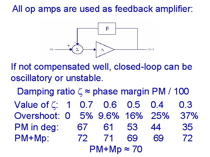
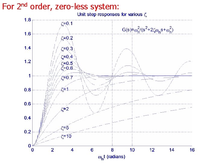
All op amps are used as feedback amplifier: If not compensated well, closed-loop can be oscillatory or unstable. Damping ratio z ≈ phase margin PM / 100 Value of z: 1 0. 7 0. 6 0. 5 0. 4 0. 3 Overshoot: 0 5% 9. 6% 16% 25% 37% PM in deg: 67 61 53 44 35 PM+Mp: 72 71 69 69 72 PM+Mp ≈ 70

For 2 nd order, zero less system:

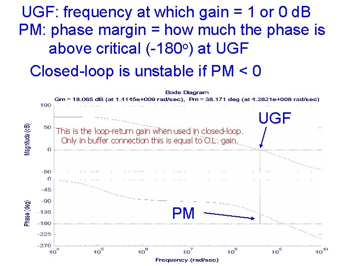
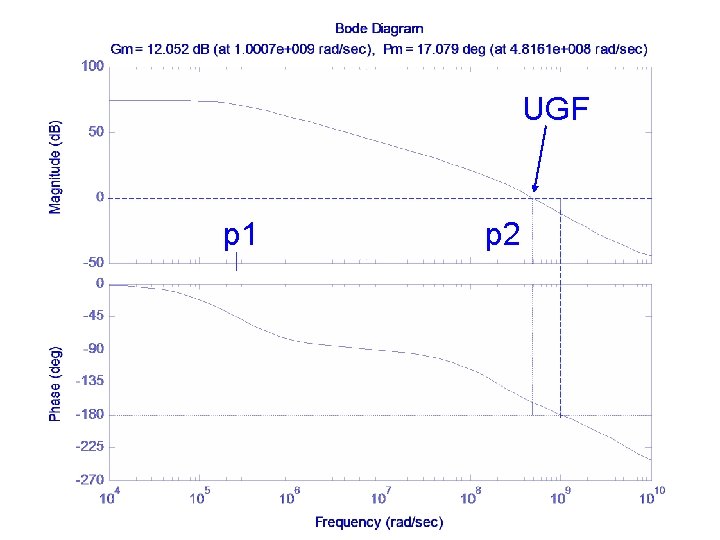
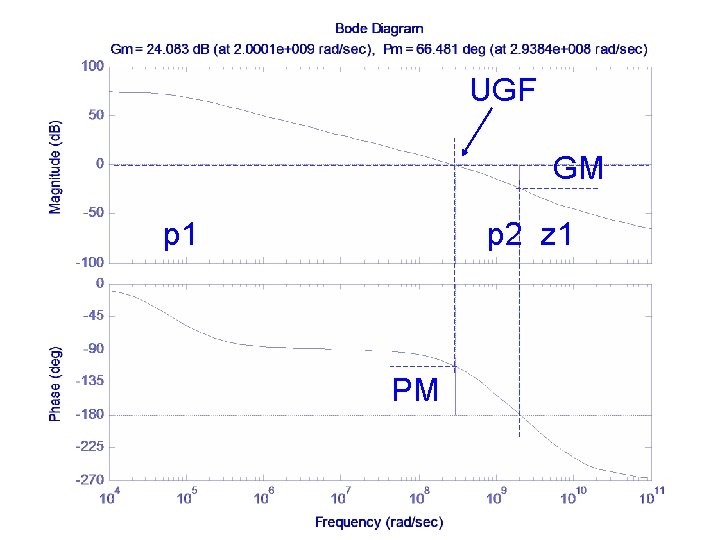
UGF: frequency at which gain = 1 or 0 d. B PM: phase margin = how much the phase is above critical (-180 o) at UGF Closed-loop is unstable if PM < 0 This is the loop return gain when used in closed loop. Only in buffer connection this is equal to O. L. gain. PM UGF

UGF p 1 p 2

UGF GM p 1 p 2 z 1 PM

Types of Compensation • Miller - Use of a capacitor feeding back around a high-gain, inverting stage. – Miller capacitor only – Miller capacitor with an unity-gain buffer to block the forward path through the compensation capacitor. Can eliminate the RHP zero. – Miller with a nulling resistor. Similar to Miller but with an added series resistance to gain control over the RHP zero. • Self compensating - Load capacitor compensates the op amp (single stage). • Feed forward - Bypassing a positive gain amplifier resulting in phase lead. Gain can be less than unity.

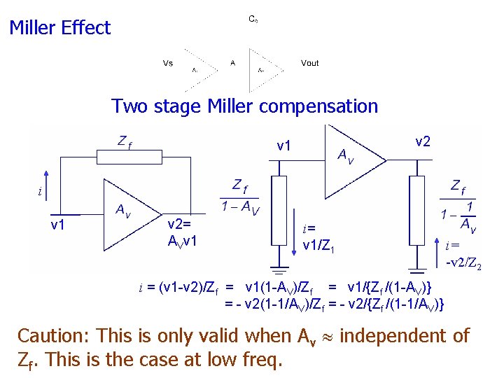
Miller Effect Two stage Miller compensation v 2 v 1 i v 1 v 2= AVv 1 i= v 1/Z 1 i= -v 2/Z 2 i = (v 1 -v 2)/Zf = v 1(1 -AV)/Zf = v 1/{Zf /(1 -AV)} = - v 2(1 -1/AV)/Zf = - v 2/{Zf /(1 -1/AV)} Caution: This is only valid when Av independent of Zf. This is the case at low freq.

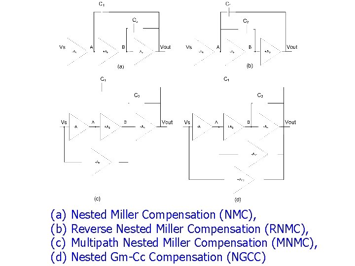
(a) (b) (c) (d) Nested Miller Compensation (NMC), Reverse Nested Miller Compensation (RNMC), Multipath Nested Miller Compensation (MNMC), Nested Gm Cc Compensation (NGCC)

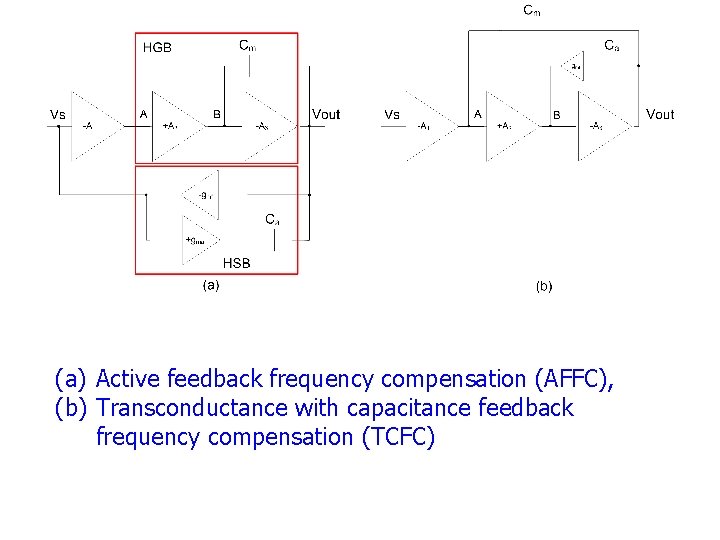
(a) Active feedback frequency compensation (AFFC), (b) Transconductance with capacitance feedback frequency compensation (TCFC)

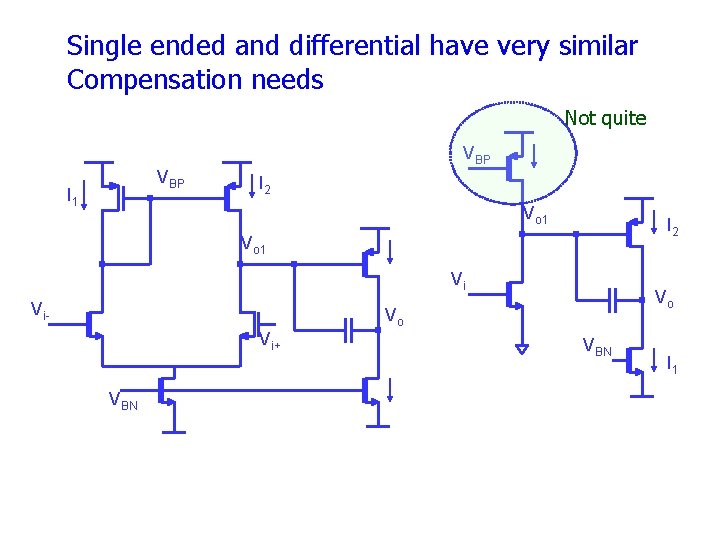
Single ended and differential have very similar Compensation needs Not quite VBP I 1 I 2 Vo 1 Vi Vi- Vo Vo Vi+ VBN I 1

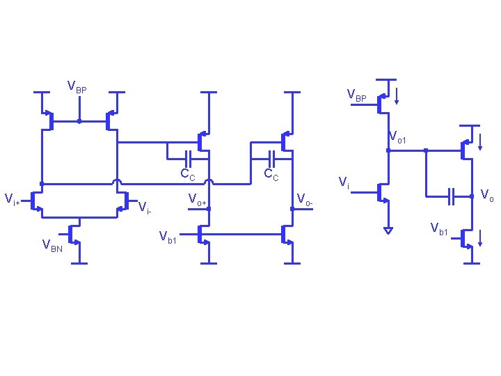
VBP Vo 1 CC Vi+ Vo+ Vi. VBN Vb 1 CC Vi Vo Vo. Vb 1

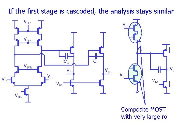
If the first stage is cascoded, the analysis stays similar VBP VBPc Vo 1 CC VBNc Vo+ Vi- Vi+ Vb 1 CC Vo- Vo Vi Vb 1 VBN Composite MOST with very large ro

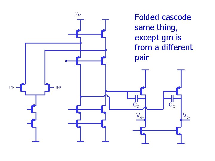
VDD IN- Folded cascode same thing, except gm is from a different pair IN+ CC Vo-

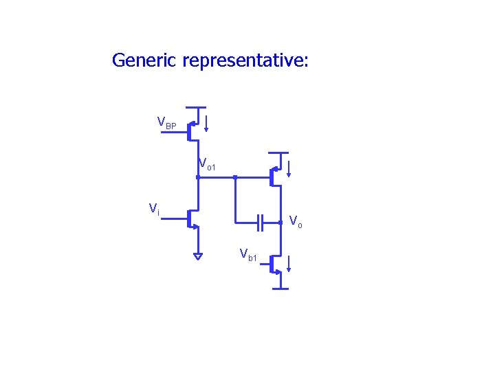
Generic representative: VBP Vo 1 Vi Vo Vb 1

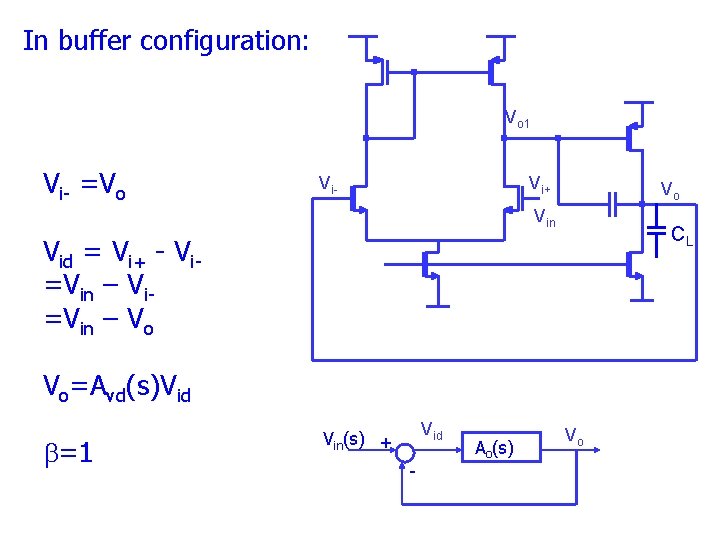
In buffer configuration: Vo 1 Vi =Vo Vi- Vi+ Vo Vin CL Vid = Vi+ Vi =Vin – Vo Vo=Avd(s)Vid b=1 Vid Vin(s) + Ao(s) Vo

Stability simulation • Perform “open loop” frequency response • Check PM at UGF • Use PM to predict overshoot in closedloop small signal step response • Need to include input impedance at vi- in total output impedance at vo.

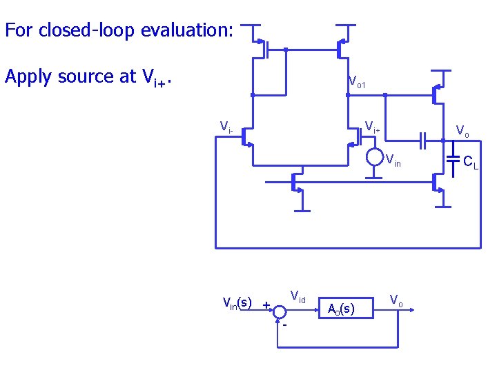
For closed loop evaluation: Apply source at Vi+. Vo 1 Vi- Vi+ Vo Vin Vid Vin(s) + Ao(s) Vo CL

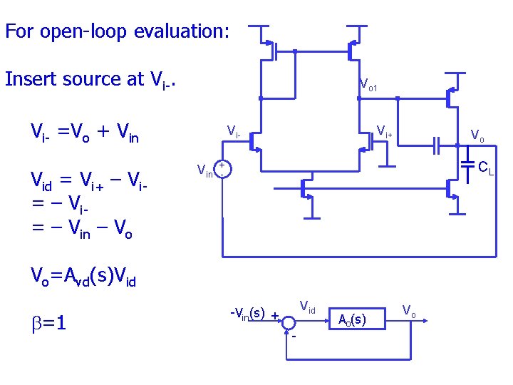
For open loop evaluation: Insert source at Vi. Vo 1 Vi =Vo + Vin Vid = Vi+ – Vi = – Vin – Vo Vi. Vin Vi+ Vo + CL Vo=Avd(s)Vid b=1 Vid Vin(s) + Ao(s) Vo

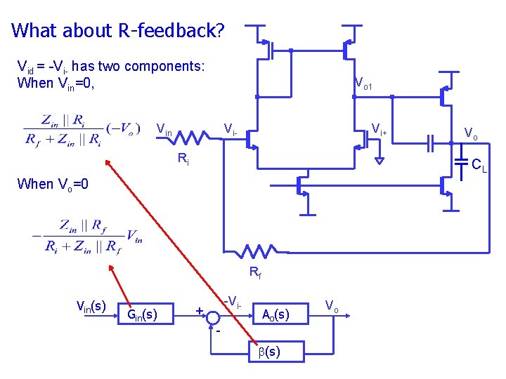
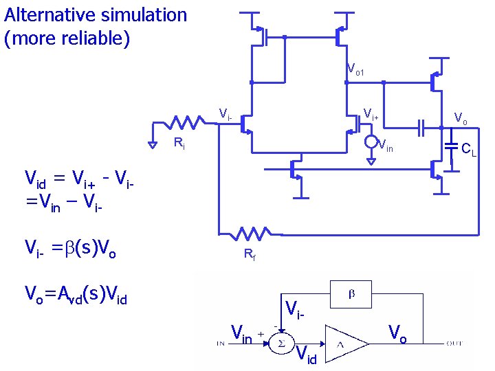
What about R feedback? Vid = -Vi- has two components: When Vin=0, Vo 1 Vin Vi- Vi+ Ri CL When Vo=0 Rf Vin(s) Gin(s) Vo -Vi- + Ao(s) b(s) Vo

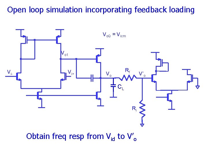
Open loop simulation incorporating feedback loading Vo. Q = Vicm Vo 1 Vi- Vi+ Rf Vo V’o CL Ri Obtain freq resp from Vid to V’o

Alternative simulation (more reliable) Vo 1 Vi- Vi+ Ri Vo Vin Vid = Vi+ Vi =Vin – Vi Vi =b(s)Vo Rf Vo=Avd(s)Vid Vin Vi Vid Vo CL

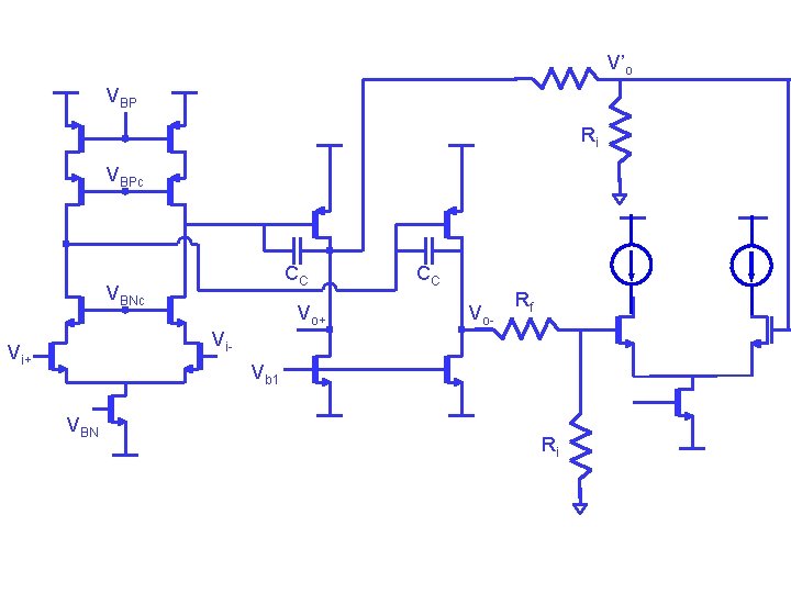
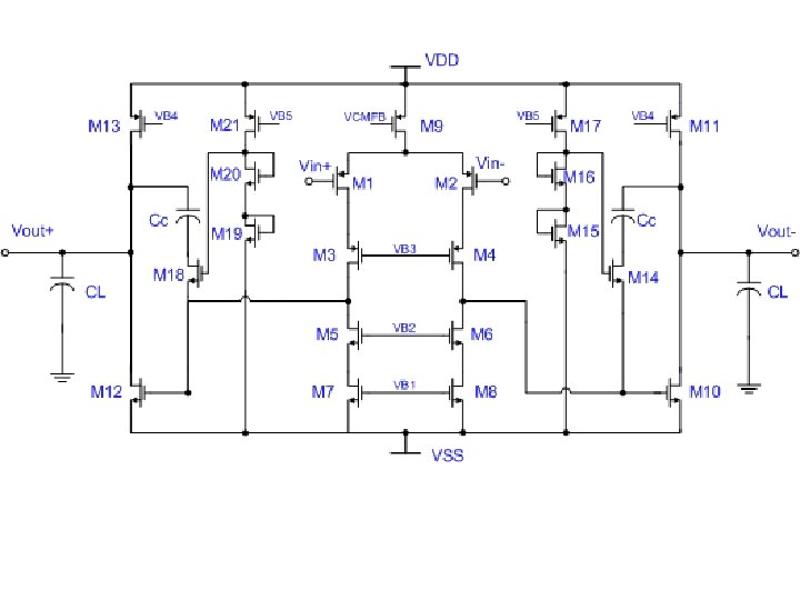
V’o VBP Ri VBPc CC VBNc Vo+ CC Vo- Rf Vi- Vi+ Vb 1 VBN Ri

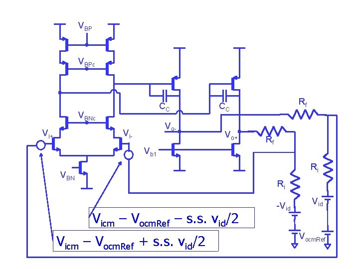
VBP VBPc CC VBNc Vi+ Vo- Vi- Rf CC Vo+ Vb 1 Rf Ri VBN Ri Vicm – Vocm. Ref – s. s. vid/2 Vicm – Vocm. Ref + s. s. vid/2 -Vid Vocm. Ref

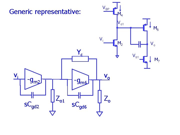
Generic representative: VBP M 4 Vo 1 Vi M 2 Yc vi gm 2 s. Cgd 2 gm 6 Zo 1 s. Cgd 6 M 6 Vo Vb 1 vo Zo M 7

Yc+s. Cgd 6 vi Io 1 s. Cgd 2 gm 2 vo 1 Zo 1 Io gm 6 Yc+s. Cgd 6 vo Zo

VBP I 1 I 2 Vo 1 Vi- Vo Vi+ VBN Yc+s. Cgd 6 Vid s. Cgd 2 V I i+ o 1 g 0. 5 m 2 Vi 0. 5 I vo 1 Zo 1 Vm Io gm 6 Yc+s. Cgd 6 vo Zo

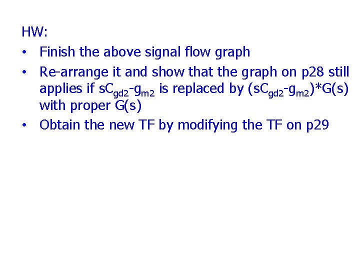
HW: • Finish the above signal flow graph • Re arrange it and show that the graph on p 28 still applies if s. Cgd 2 gm 2 is replaced by (s. Cgd 2 gm 2)*G(s) with proper G(s) • Obtain the new TF by modifying the TF on p 29

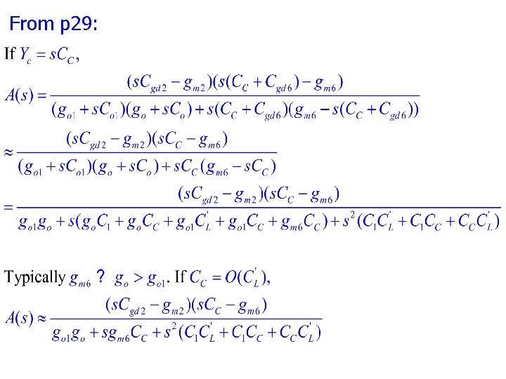
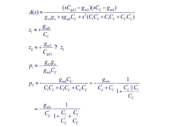
From p 29:

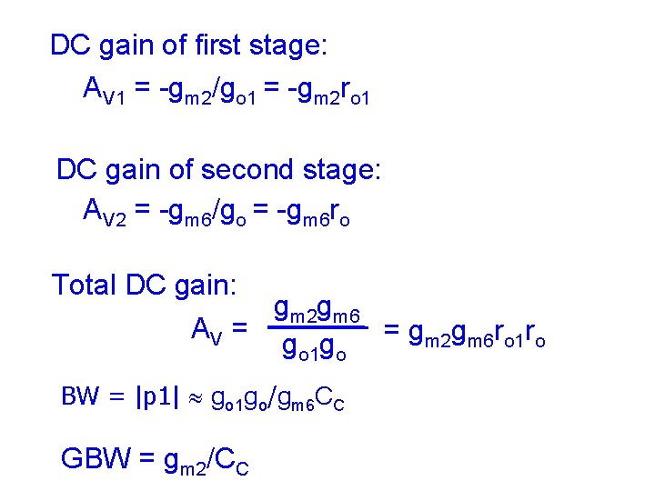
DC gain of first stage: AV 1 = -gm 2/go 1 = -gm 2 ro 1 DC gain of second stage: AV 2 = -gm 6/go = -gm 6 ro Total DC gain: gm 2 gm 6 AV = = g g r r m 2 m 6 o 1 o go 1 go BW = |p 1| go 1 go/gm 6 CC GBW = gm 2/CC

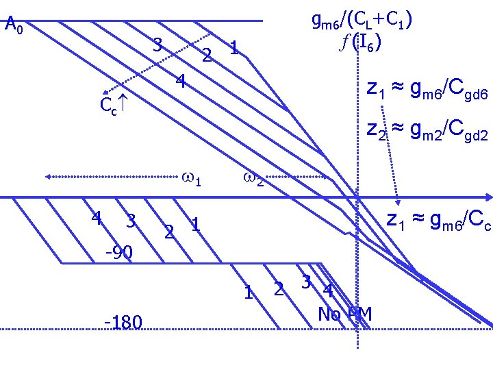
gm 6/(CL+C 1) f (I 6) A 0 z 1 ≈ gm 6/(CC+Cgd 6) w 1 0 d. B 90 w 2 z 2 ≈ gm 2/Cgd 2 o 180 o No PM

A 0 3 C c 2 1 4 3 90 z 1 ≈ gm 6/Cgd 6 z 2 ≈ gm 2/Cgd 2 w 1 4 gm 6/(CL+C 1) f (I 6) w 2 z 1 ≈ gm 6/Cc 2 1 1 180 2 3 4 No PM

gm 6/(CL+C 1) f (I 6) A 0 gm 1/CC w 2 w 1 90 180 PM z 1 ≈ gm 6/CC

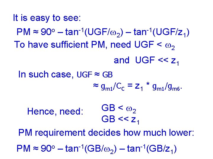
It is easy to see: PM ≈ 90 o – tan-1(UGF/w 2) – tan-1(UGF/z 1) To have sufficient PM, need UGF < w 2 and UGF << z 1 In such case, UGF ≈ GB ≈ gm 1/CC = z 1 * gm 1/gm 6. GB < w 2 GB << z 1 PM requirement decides how much lower: Hence, need: PM ≈ 90 o – tan-1(GB/w 2) – tan-1(GB/z 1)

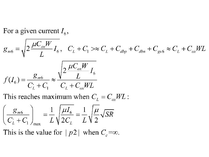
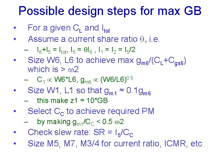
Possible design steps for max GB • • For a given CL and Itot Assume a current share ratio q, i. e. – • Size W 6, L 6 to achieve max gm 6/(CL+Cgs 6) which is > w 2 – • this make z 1 ≈ 10*GB Select CC to achieve required PM – • • C 1 W 6*L 6, gm 6 (W 6/L 6)0. 5 Size W 1, L 1 so that gm 1 ≈ 0. 1 gm 6 – • I 6+I 5 = Itot, I 5 = q. I 6 , I 1 = I 2 = I 5/2 by making gm 1/CC < 0. 5 w 2 Check slew rate: SR = I 5/CC Size M 5, M 7, M 3/4 for current ratio, ICMR, etc

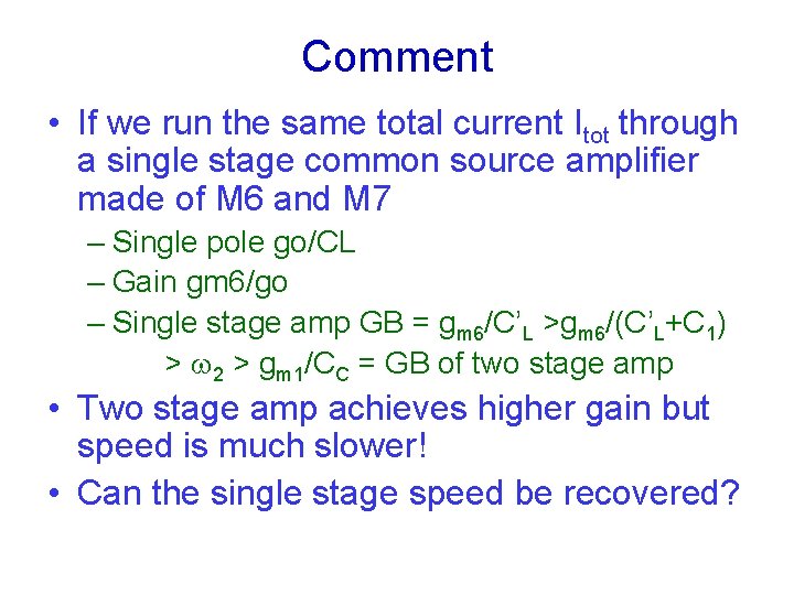
Comment • If we run the same total current Itot through a single stage common source amplifier made of M 6 and M 7 – Single pole go/CL – Gain gm 6/go – Single stage amp GB = gm 6/C’L >gm 6/(C’L+C 1) > w 2 > gm 1/CC = GB of two stage amp • Two stage amp achieves higher gain but speed is much slower! • Can the single stage speed be recovered?

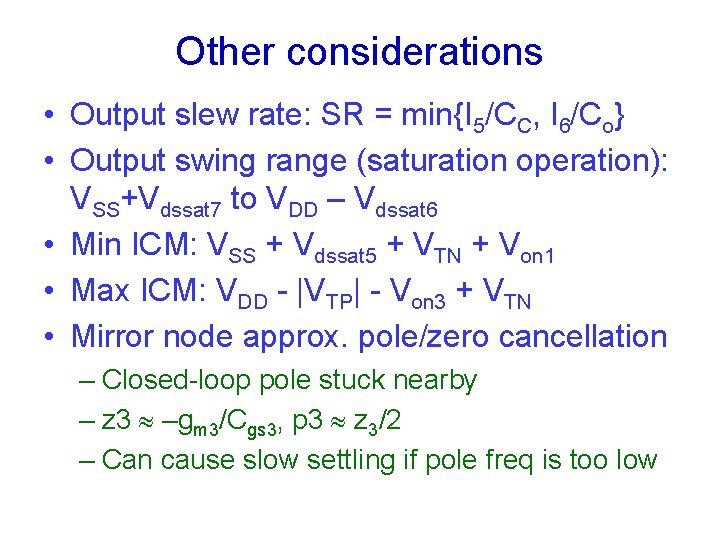
Other considerations • Output slew rate: SR = min{I 5/CC, I 6/Co} • Output swing range (saturation operation): VSS+Vdssat 7 to VDD – Vdssat 6 • Min ICM: VSS + Vdssat 5 + VTN + Von 1 • Max ICM: VDD - |VTP| - Von 3 + VTN • Mirror node approx. pole/zero cancellation – Closed-loop pole stuck nearby – z 3 –gm 3/Cgs 3, p 3 z 3/2 – Can cause slow settling if pole freq is too low

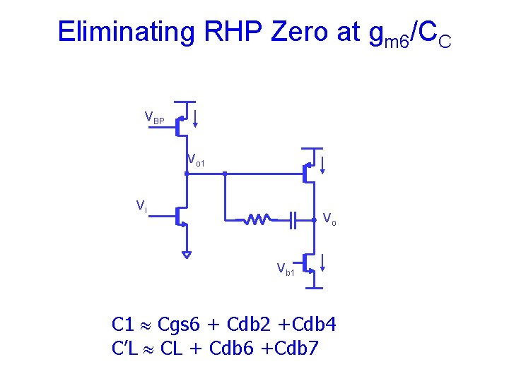
Eliminating RHP Zero at gm 6/CC VBP Vo 1 Vi Vo Vb 1 C 1 Cgs 6 + Cdb 2 +Cdb 4 C’L CL + Cdb 6 +Cdb 7

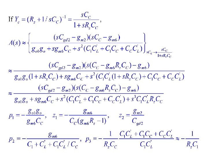
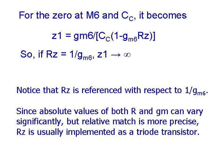
For the zero at M 6 and CC, it becomes z 1 = gm 6/[CC(1 -gm 6 Rz)] So, if Rz = 1/gm 6, z 1 → Notice that Rz is referenced with respect to 1/gm 6. Since absolute values of both R and gm can vary significantly, but relative match is more precise, Rz is usually implemented as a triode transistor.

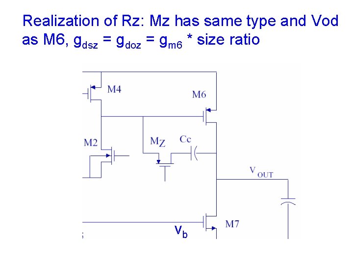
Realization of Rz: Mz has same type and Vod as M 6, gdsz = gdoz = gm 6 * size ratio vb

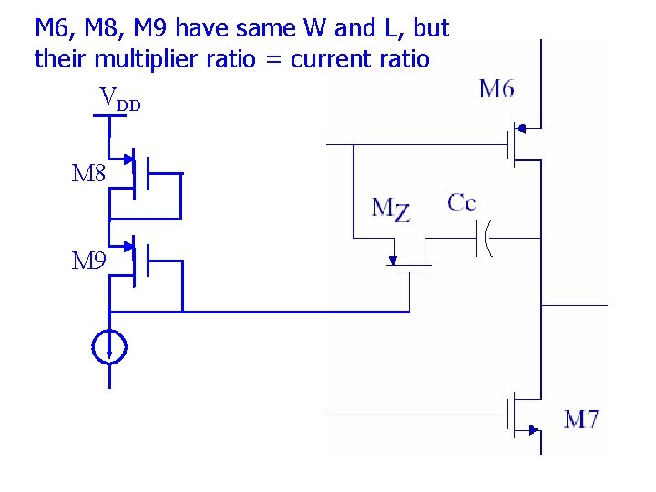
M 6, M 8, M 9 have same W and L, but their multiplier ratio = current ratio VDD M 8 M 9

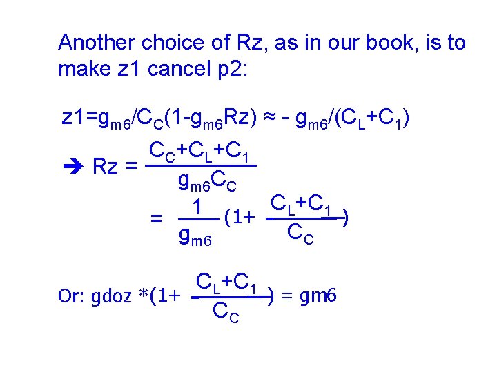
Another choice of Rz, as in our book, is to make z 1 cancel p 2: z 1=gm 6/CC(1 -gm 6 Rz) ≈ - gm 6/(CL+C 1) CC+CL+C 1 Rz = gm 6 CC 1 (1+ CL+C 1 ) = CC gm 6 CL+C 1 ) = gm 6 Or: gdoz * (1+ CC

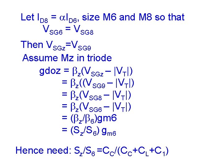
Let ID 8 = a. ID 6, size M 6 and M 8 so that VSG 6 = VSG 8 Then VSGz=VSG 9 Assume Mz in triode gdoz = bz(VSGz – |VT|) = bz((VSG 9 – |VT|) = bz(VSG 8 – |VT|) = bz(VSG 6 – |VT|) = (bz/b 6)gm 6 = (Sz/S 6) gm 6 Hence need: Sz/S 6 =CC/(CC+CL+C 1)

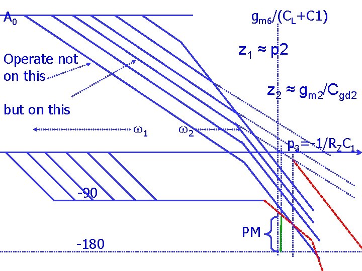
gm 6/(CL+C 1) A 0 z 1 ≈ p 2 Operate not on this z 2 ≈ gm 2/Cgd 2 but on this w 1 w 2 p 3= 1/RZC 1 90 180 PM

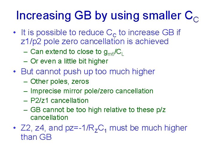
Increasing GB by using smaller CC • It is possible to reduce CC to increase GB if z 1/p 2 pole zero cancellation is achieved – Can extend to close to gm 6/CL – Or even a little bit higher • But cannot push up too much higher – – Other poles, zeros Imprecise mirror pole/zero cancellation P 2/z 1 cancellation GB cannot be too high relative to these p/z cancellation • Z 2, z 4, and pz=-1/RZC 1 must be much higher than GB

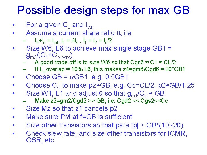
Possible design steps for max GB • • For a given CL and Itot Assume a current share ratio q, i. e. – • – – • • I 6+I 5 = Itot, I 5 = q. I 6 , I 1 = I 2 = I 5/2 Size W 6, L 6 to achieve max single stage GB 1 = gm 6/(CL+Co-para) A good trade off is to size W 6 so that Cgs 6 ≈ C 1 ≈ CL/2 If L_overlap ≈ 10% L 6, this makes z 4=gm 6/Cgd 6 ≈ 20*GB 1 Choose GB = a. GB 1, e. g. 0. 5 GB 1 Choose CC to make p 2≈GB, e. g. Cc=CL/2, p 2≈GB/1. 25 Size W 1, L 1 and adjust q so that gm 1/CC ≈ GB Make z 2=gm 2/Cgd 2 >> GB, i. e. Cgd 2 << Cgs 2<<Cc Size Mz so that z 1 cancels p 2 Make sure PM at f=GB is sufficient Size other transistors so that para |p| > GB*(10~20) Check slew rate, and size other transistors for ICMR, OSR, etc

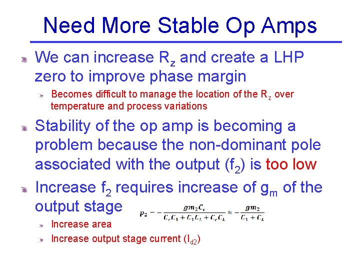
Need More Stable Op Amps We can increase Rz and create a LHP zero to improve phase margin Becomes difficult to manage the location of the Rz over temperature and process variations Stability of the op amp is becoming a problem because the non-dominant pole associated with the output (f 2) is too low Increase f 2 requires increase of gm of the output stage Increase area Increase output stage current (Id 2)

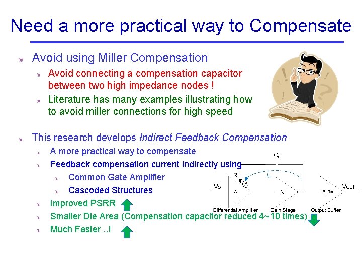
Need a more practical way to Compensate Avoid using Miller Compensation Avoid connecting a compensation capacitor between two high impedance nodes ! Literature has many examples illustrating how to avoid miller connections for high speed This research develops Indirect Feedback Compensation A more practical way to compensate Feedback compensation current indirectly using Common Gate Amplifier Cascoded Structures Improved PSRR Smaller Die Area (Compensation capacitor reduced 4~10 times) Much Faster. . !

Indirect Feedback - History • First proposed by B. K. Ahuja in “AN IMPROVED FREQUENCY COMPENSATION TECHNIQUE FOR CMOS OPERATIONAL-AMPLIFIERS, ” Ieee Journal of Solid-State Circuits, vol. 18, no. 6, pp. 629 -633, 1983 • However it is still seldom used in practice ? ? – Looks very similar to Miller compensation – Prompts most designers to use design strategy for Miller-Rz compensation – However the Indirect Compensation Scheme has different pole/zero locations and conditions that need to be satisfied to tap the true potential of the compensation scheme – Thus this work Provides analytical model/solution for the architecture Proposes a design procedure based on the analytical results Design Example using the proposed design procedure Simulation Results show the performance is orders of magnitude higher than miller compensation and far better than state of the art

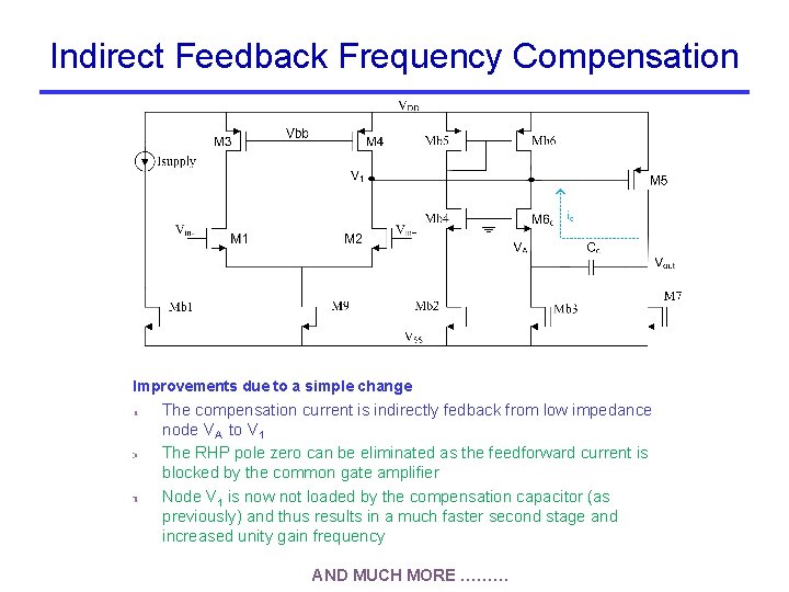
Indirect Feedback Frequency Compensation Improvements due to a simple change The compensation current is indirectly fedback from low impedance node VA to V 1 The RHP pole zero can be eliminated as the feedforward current is blocked by the common gate amplifier Node V 1 is now not loaded by the compensation capacitor (as previously) and thus results in a much faster second stage and increased unity gain frequency AND MUCH MORE ………

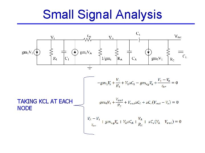
Small Signal Analysis TAKING KCL AT EACH NODE

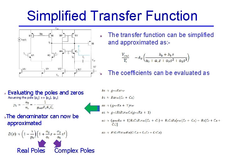
Simplified Transfer Function The transfer function can be simplified and approximated as: - The coefficients can be evaluated as Evaluating the poles and zeros Assuming the pole |p 1| >> |p 2|, |p 3| The denominator can now be approximated Real Poles Complex Poles

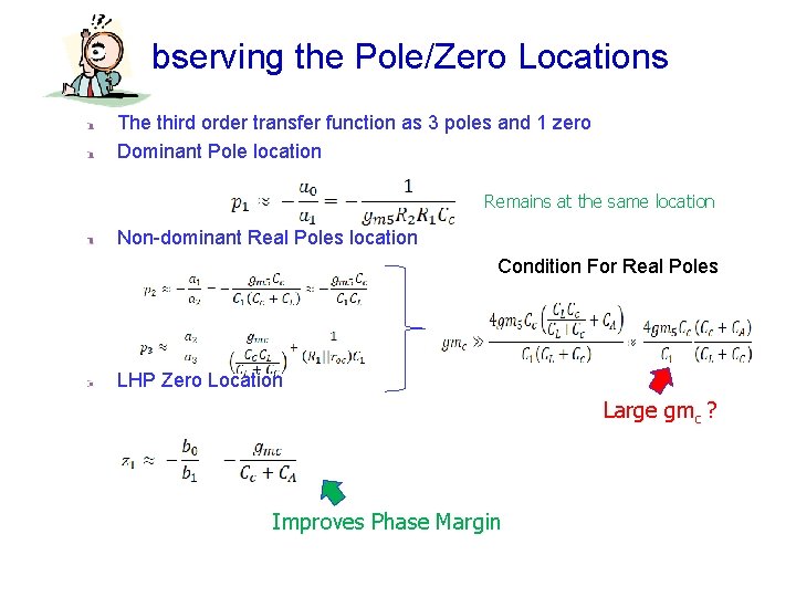
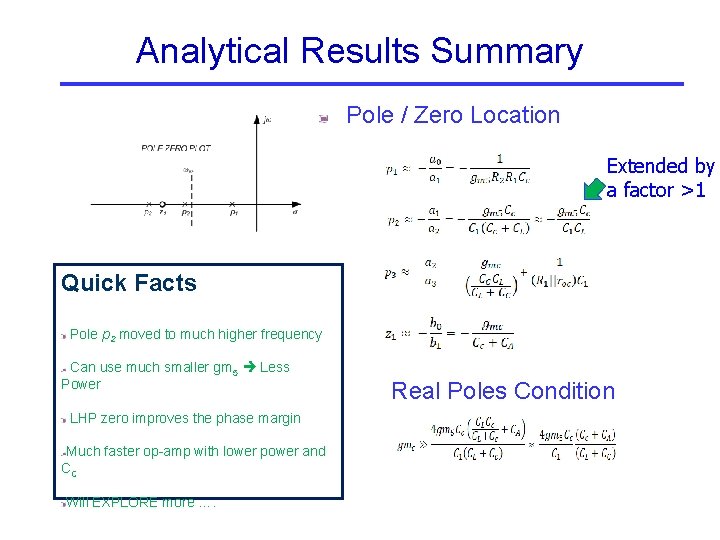
bserving the Pole/Zero Locations The third order transfer function as 3 poles and 1 zero Dominant Pole location Remains at the same location Non-dominant Real Poles location Condition For Real Poles LHP Zero Location Large gmc ? Improves Phase Margin

Analytical Results Summary Pole / Zero Location Extended by a factor >1 Quick Facts Pole p 2 moved to much higher frequency Can use much smaller gm 5 Less Power LHP zero improves the phase margin Much faster op-amp with lower power and CC Will EXPLORE more …. Real Poles Condition

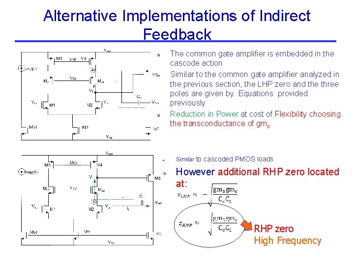
Alternative Implementations of Indirect Feedback The common gate amplifier is embedded in the cascode action Similar to the common gate amplifier analyzed in the previous section, the LHP zero and the three poles are given by Equations provided previously Reduction in Power at cost of Flexibility choosing the transconductance of gmc Similar to cascoded PMOS loads However additional RHP zero located at: RHP zero High Frequency

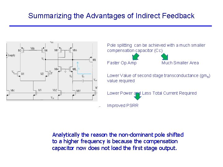
Summarizing the Advantages of Indirect Feedback Pole splitting can be achieved with a much smaller compensation capacitor (Cc) Faster Op Amp Much Smaller Area Lower Value of second stage transconductance (gm 5) value required Lower Power and Less Total Current Required Improved PSRR Analytically the reason the non dominant pole shifted to a higher frequency is because the compensation capacitor now does not load the first stage output.

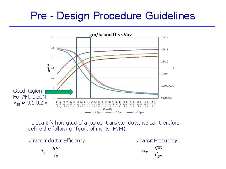
Pre - Design Procedure Guidelines Good Region For AMI 0. 5 CN VEB ≈ 0. 1 0. 2 V To quantify how good of a job our transistor does, we can therefore define the following “figure of merits (FOM) Tranconductor Efficiency Transit Frequency

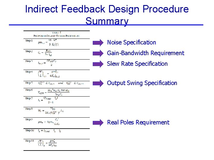
Indirect Feedback Design Procedure Summary Noise Specification Gain Bandwidth Requirement Slew Rate Specification Output Swing Specification Real Poles Requirement

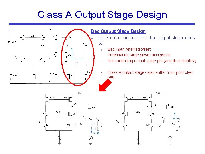
Class A Output Stage Design Bad Output Stage Design Not Controlling current in the output stage leads to: Bad input-referred offset Potential for large power dissipation Not controlling output stage gm (and thus stability) Class A output stages also suffer from poor slew rate

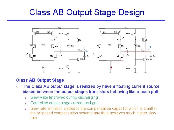
Class AB Output Stage Design Class AB Output Stage The Class AB output stage is realized by have a floating current source biased between the output stages transistors behaving like a push pull: Slew Rate Improved during discharging Controlled output stage current and gm Slew rate limitation shifted to the compensation capacitor which is small in the proposed compensation scheme and thus achieves much higher slew rate

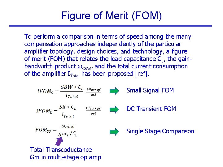
Figure of Merit (FOM) To perform a comparison in terms of speed among the many compensation approaches independently of the particular amplifier topology, design choices, and technology, a figure of merit (FOM) that relates the load capacitance CL, the gain bandwidth product ωGBW, and the total current consumption of the amplifier I Total has been proposed [ref]. Small Signal FOM DC Transient FOM Single Stage Comparison Total Transcoductance Gm in multi stage op amp

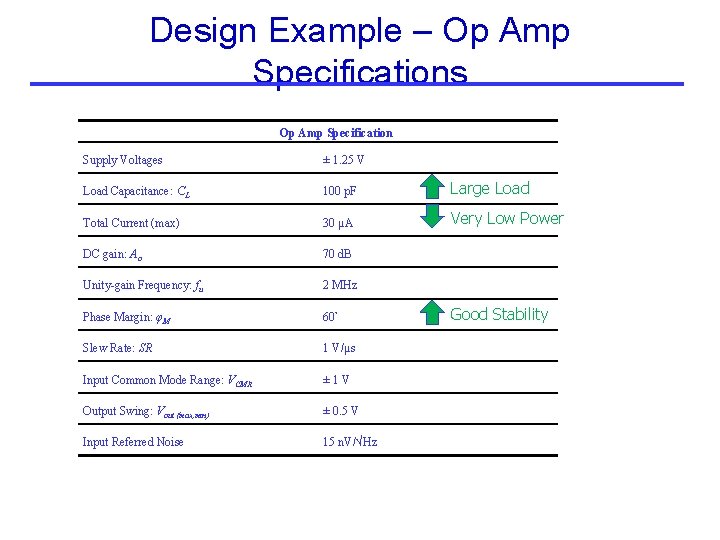
Design Example – Op Amp Specifications Op Amp Specification Supply Voltages ± 1. 25 V Load Capacitance: CL 100 p. F Large Load Total Current (max) 30 μA Very Low Power DC gain: Ao 70 d. B Unity-gain Frequency: fu 2 MHz Phase Margin: φM 60° Slew Rate: SR 1 V/μs Input Common Mode Range: VCMR ± 1 V Output Swing: Vout {max, min} ± 0. 5 V Input Referred Noise 15 n. V/√Hz Good Stability

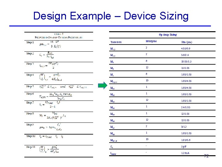
Design Example – Device Sizing Op Amp Sizing Transistor Multiplier Size (μm) M 1, 2 2 4. 05/0. 9 M 3, 4 2 3. 6/2. 4 M 5 6 10. 05/1. 5 M 6 12 15/1. 05 M 7 6 1. 65/1. 05 M 9, b 11 10 1. 65/4. 05 Mb 1 1 1. 65/4. 05 Mb 2 1 1. 65/1. 05 Mb 3 12 1. 65/1. 05 Mb 4 1 2. 4/1. 05 Mb 5 1 12/1. 05 Mb 6 12 12/1. 05 Mb 7 2 3/1. 2 Mb 8 1 1. 65/1. 05 Mb 9, 10 10 1. 95/0. 6 Cc - 5 p. F Isupply - 1. 25 u. A 72

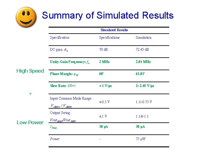
Summary of Simulated Results High Speed Specifications Simulation DC gain: Ao 70 d. B 72. 45 d. B Unity-Gain Frequency: fu 2 MHz 2. 01 MHz Phase Margin: φM 60° 61. 83° Slew Rate: SR+/- ± 1 V/μs 1/-2. 45 V/μs ± 0. 5 V 1. 1/-0. 75 V ± 1 V 1. 14/-1. 1 ITotal 30 μA Power - 75 μW + Input Common Mode Range: VCMR + / VCMR= Output Swing: Low Power Vout MAX/Vout MIN

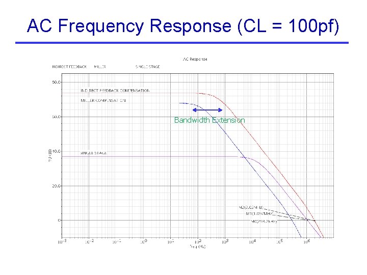
AC Frequency Response (CL = 100 pf) Bandwidth Extension

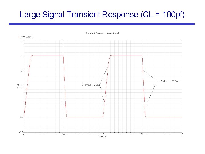
Large Signal Transient Response (CL = 100 pf)

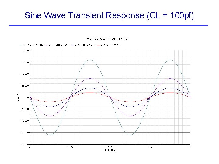
Sine Wave Transient Response (CL = 100 pf)

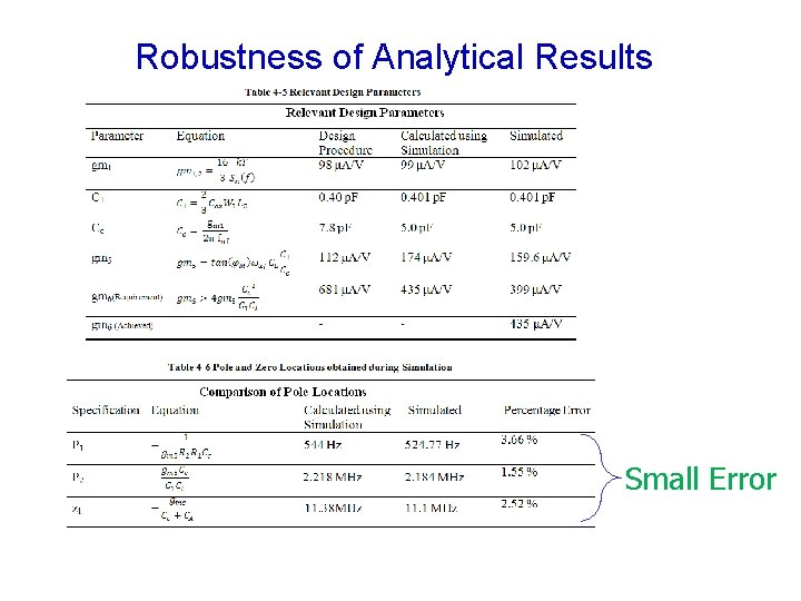
Robustness of Analytical Results Small Error

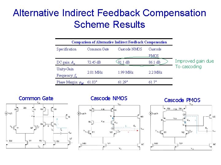
Alternative Indirect Feedback Compensation Scheme Results Comparison of Alternative Indirect Feedback Compensation Specification Common Gate Cascode NMOS Cascode PMOS DC gain: Ao Unity-Gain Frequency: fu Phase Margin: φM Common Gate 72. 45 d. B 91. 1 d. B 86. 1 d. B 2. 01 MHz 1. 99 MHz 2. 2 MHz 61. 83˚ 61. 29˚ 61. 7˚ Cascode NMOS Improved gain due To cascoding Cascode PMOS

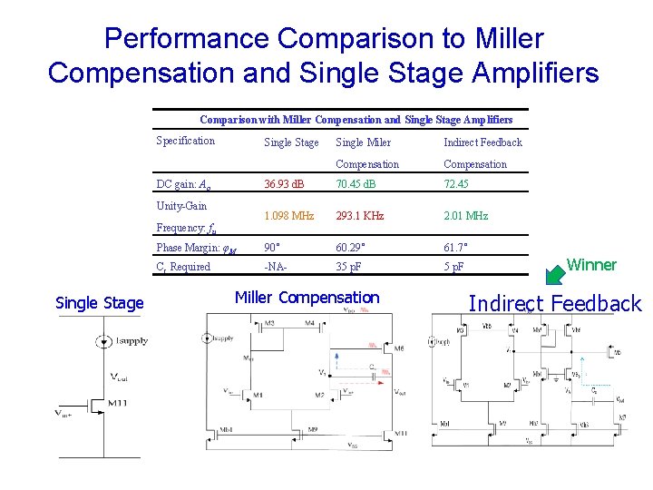
Performance Comparison to Miller Compensation and Single Stage Amplifiers Comparison with Miller Compensation and Single Stage Amplifiers Specification Single Stage Single Miler Indirect Feedback Compensation 36. 93 d. B 70. 45 d. B 72. 45 1. 098 MHz 293. 1 KHz 2. 01 MHz Phase Margin: φM 90˚ 60. 29˚ 61. 7˚ Cc Required -NA- 35 p. F DC gain: Ao Unity-Gain Frequency: fu Single Stage Miller Compensation Winner Indirect Feedback

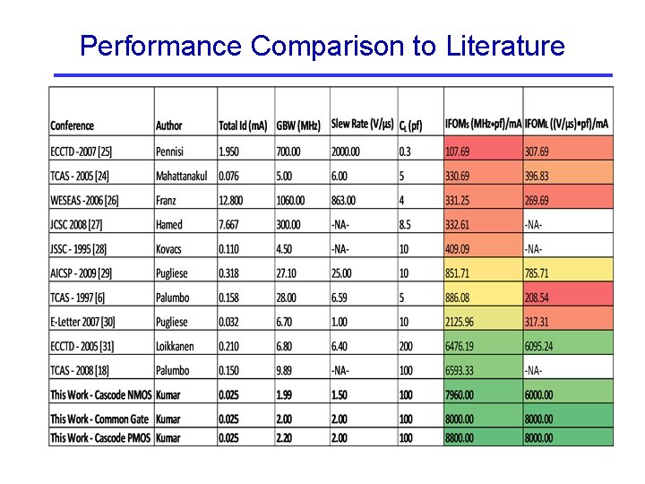
Performance Comparison to Literature

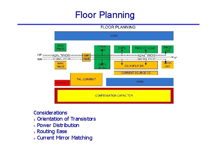
Floor Planning Considerations Orientation of Transistors Power Distribution Routing Ease Current Mirror Matching

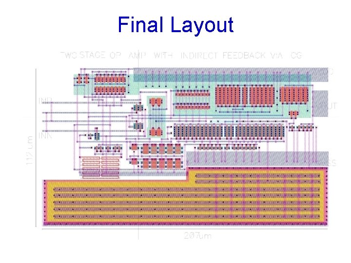
Final Layout