Propagating Functional Dependencies with Conditions Wenfei Fan University

Propagating Functional Dependencies with Conditions Wenfei Fan University of Edinburgh & Bell Laboratories Shuai Ma University of Edinburgh Yanli Hu National University of Defense Technology Jie Liu Chinese Academy of Sciences Yinghui Wu University of Edinburgh 1

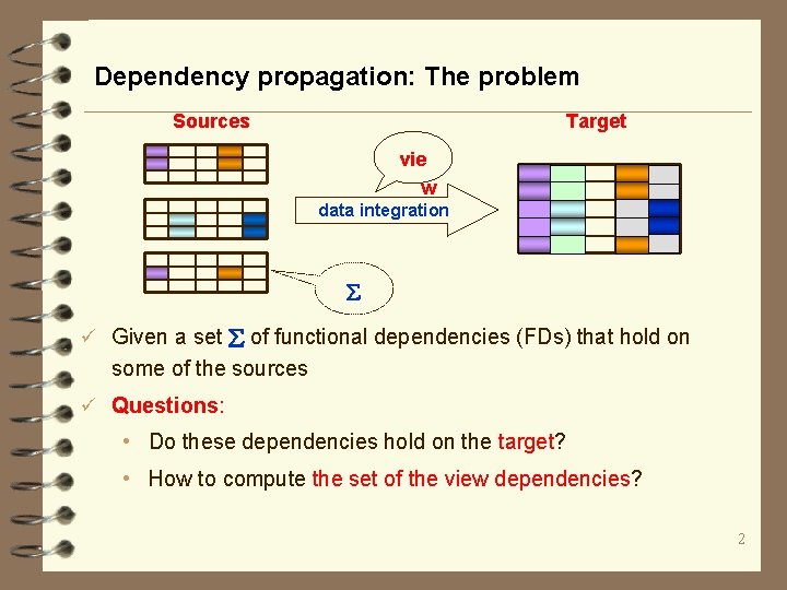
Dependency propagation: The problem Sources Target vie w data integration ü Given a set of functional dependencies (FDs) that hold on some of the sources ü Questions: • Do these dependencies hold on the target? • How to compute the set of the view dependencies? 2

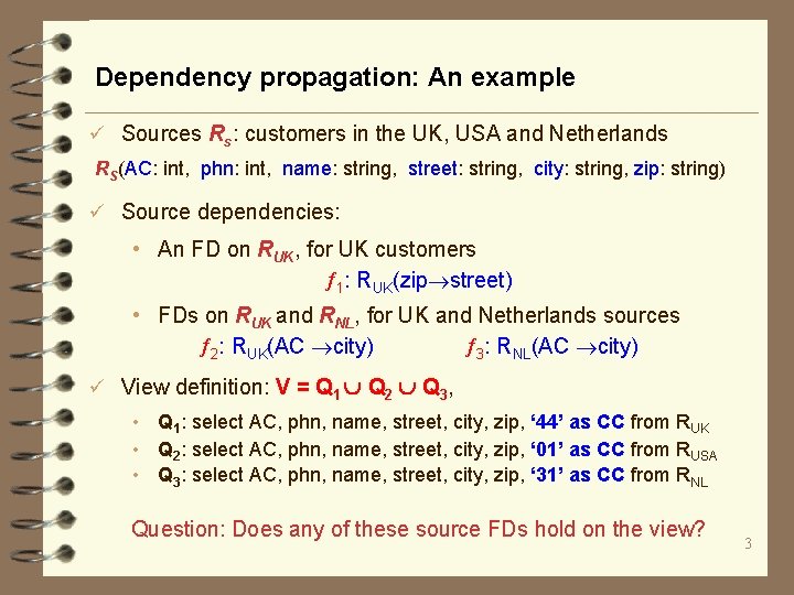
Dependency propagation: An example ü Sources Rs: customers in the UK, USA and Netherlands RS(AC: int, phn: int, name: string, street: string, city: string, zip: string) ü Source dependencies: • An FD on RUK, for UK customers 1: RUK(zip street) • FDs on RUK and RNL, for UK and Netherlands sources 2: RUK(AC city) 3: RNL(AC city) ü View definition: V = Q 1 Q 2 Q 3, • Q 1: select AC, phn, name, street, city, zip, ‘ 44’ as CC from RUK • Q 2: select AC, phn, name, street, city, zip, ‘ 01’ as CC from RUSA • Q 3: select AC, phn, name, street, city, zip, ‘ 31’ as CC from RNL Question: Does any of these source FDs hold on the view? 3

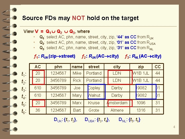
Source FDs may NOT hold on the target View V = Q 1 Q 2 Q 3, where • • • Q 1: select AC, phn, name, street, city, zip, ‘ 44’ as CC from RUK Q 2: select AC, phn, name, street, city, zip, ‘ 01’ as CC from RUSA Q 3: select AC, phn, name, street, city, zip, ‘ 31’ as CC from RNL 1: RUK(zip street) t 1 : t 2 : t 3 : t 4 : t 5 : t 6 : 2: RUK(AC city) 3: RNL(AC city) AC phn name street city zip CC 20 1234567 Mike Portland LDN W 1 B 1 JL 44 20 3456789 Rick Portland LDN W 1 B 1 JL 44 610 3456789 Joe Copley Darby 19082 01 610 1234567 Mary Walnut Darby 19082 01 20 3456789 Marx Kruise Amsterdam 1096 31 36 1234567 Bart Grote Almere 1316 31 DUK: {t 1, t 2}, DUSA: {t 3, t 4}, DNL: {t 5, t 6} 4

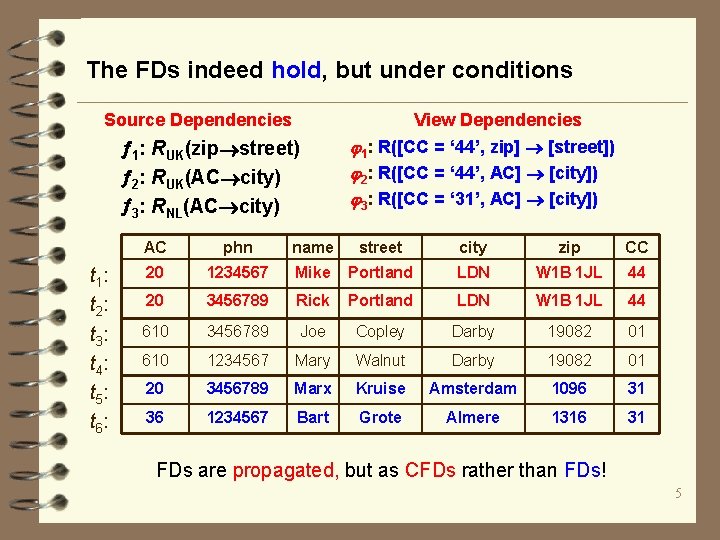
The FDs indeed hold, but under conditions Source Dependencies View Dependencies 1: R([CC = ‘ 44’, zip] [street]) 2: R([CC = ‘ 44’, AC] [city]) 3: R([CC = ‘ 31’, AC] [city]) 1: RUK(zip street) 2: RUK(AC city) 3: RNL(AC city) AC phn name street city zip CC t 1 : t 2 : 20 1234567 Mike Portland LDN W 1 B 1 JL 44 20 3456789 Rick Portland LDN W 1 B 1 JL 44 t 3 : t 4 : t 5 : t 6 : 610 3456789 Joe Copley Darby 19082 01 610 1234567 Mary Walnut Darby 19082 01 20 3456789 Marx Kruise Amsterdam 1096 31 36 1234567 Bart Grote Almere 1316 31 FDs are propagated, but as CFDs rather than FDs! 5

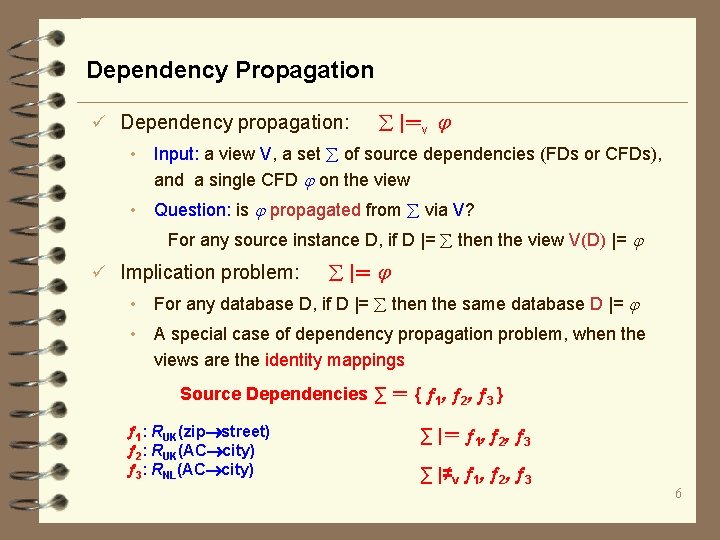
Dependency Propagation ü Dependency propagation: |＝v • Input: a view V, a set of source dependencies (FDs or CFDs), and a single CFD on the view • Question: is propagated from via V? For any source instance D, if D |= then the view V(D) |= ü Implication problem: |＝ • For any database D, if D |= then the same database D |= • A special case of dependency propagation problem, when the views are the identity mappings Source Dependencies ∑ ＝ { 1, 2, 3 } 1: RUK(zip street) 2: RUK(AC city) 3: RNL(AC city) ∑ |＝ 1, 2, 3 ∑ |≠v 1, 2, 3 6

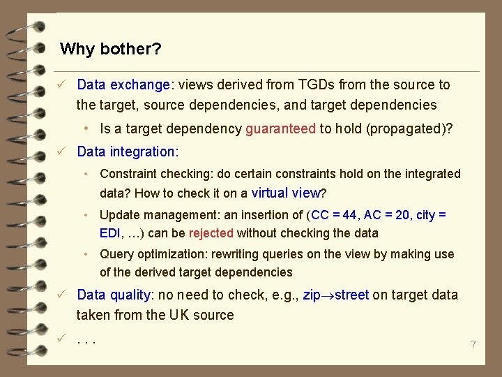
Why bother? ü Data exchange: views derived from TGDs from the source to the target, source dependencies, and target dependencies • Is a target dependency guaranteed to hold (propagated)? ü Data integration: • Constraint checking: do certain constraints hold on the integrated data? How to check it on a virtual view? • Update management: an insertion of (CC = 44, AC = 20, city = EDI, …) can be rejected without checking the data • Query optimization: rewriting queries on the view by making use of the derived target dependencies ü Data quality: no need to check, e. g. , zip street on target data taken from the UK source ü. . . 7

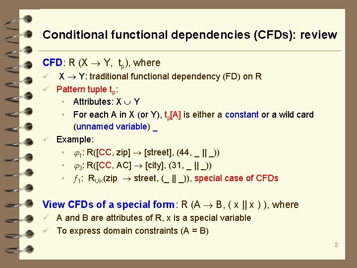
Conditional functional dependencies (CFDs): review CFD: R (X Y, tp), where X Y: traditional functional dependency (FD) on R ü Pattern tuple tp: • Attributes: X Y • For each A in X (or Y), tp[A] is either a constant or a wild card (unnamed variable) _ ü Example: • 1: R([CC, zip] [street], (44, _ || _)) • 3: R([CC, AC] [city], (31, _ || _)) • 1: RUK(zip street, (_ || _)), special case of CFDs ü View CFDs of a special form: R (A B, ( x || x ) ), where ü A and B are attributes of R, x is a special variable ü To express domain constraints (A = B) 8

View definitions: A brief overview A relational Schema = {S 1, … , Sn} ü SPC query Q = ∏Y(Rc x Es), where • Rc = {(A 1: a 1, … Am: am)} • Es = σF(R 1 x … x Rn) § F is a conjunction of equality atoms of the form A = B and A = ‘a’ for a constant ‘a’ in dom(A) § Rj is ρ(S) for some S in ü SPCU query Q = V 1 … Vn , where • Vi is an SPC query ü Example • Q 1 = {(CC : 44)} x RUK, Q 2 = {(CC : 01)} x RUSA, Q 3 = {(CC : 31)} x RNL • R = Q 1 Q 2 Q 3 9

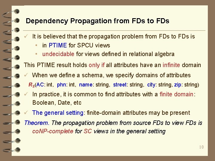
Dependency Propagation from FDs to FDs ü It is believed that the propagation problem from FDs to FDs is • in PTIME for SPCU views • undecidable for views defined in relational algebra This PTIME result holds only if all attributes have an infinite domain ü When we define a schema, we specify domains of attributes RS(AC: int, phn: int, name: string, street: string, city: string, zip: string) ü In practice, it is common to find attributes with a finite domain: Boolean, Date, etc ü The general setting: finite-domain attributes may be present Theorem. The propagation problem from source FDs to view FDs is co. NP-complete for SC views in the general setting 10

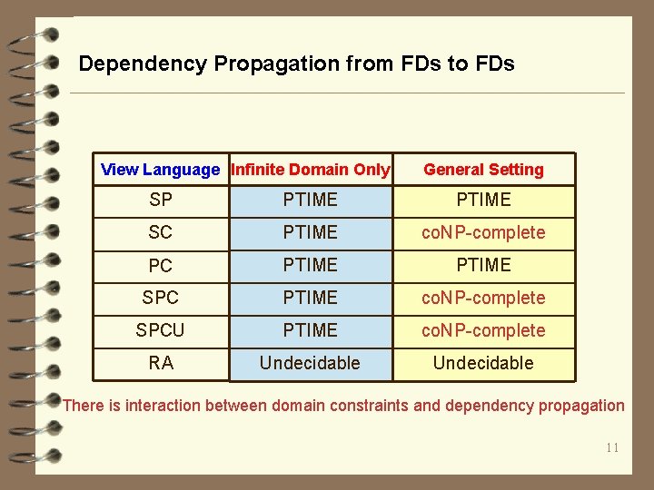
Dependency Propagation from FDs to FDs View Language Infinite Domain Only General Setting SP PTIME SC PTIME co. NP-complete PC PTIME SPC PTIME co. NP-complete SPCU PTIME co. NP-complete RA Undecidable There is interaction between domain constraints and dependency propagation 11

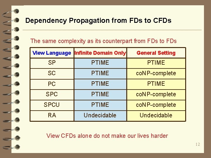
Dependency Propagation from FDs to CFDs The same complexity as its counterpart from FDs to FDs View Language Infinite Domain Only General Setting SP PTIME SC PTIME co. NP-complete PC PTIME SPC PTIME co. NP-complete SPCU PTIME co. NP-complete RA Undecidable View CFDs alone do not make our lives harder 12

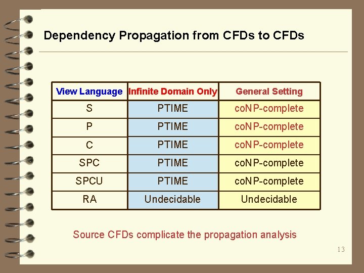
Dependency Propagation from CFDs to CFDs View Language Infinite Domain Only General Setting S PTIME co. NP-complete P PTIME co. NP-complete C PTIME co. NP-complete SPCU PTIME co. NP-complete RA Undecidable Source CFDs complicate the propagation analysis 13

Propagation Cover Problem Sources Target vie w data integration c Problem Statement ü Input: • a view V • a set of source dependencies (CFDs) ü Output: A propagation cover c a cover of all view CFDs propagated from via V 14

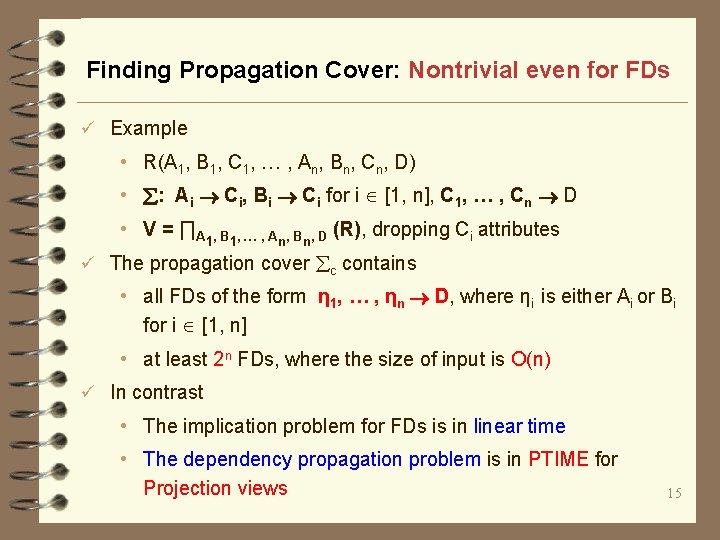
Finding Propagation Cover: Nontrivial even for FDs ü Example • R(A 1, B 1, C 1, … , An, Bn, Cn, D) • : Ai Ci, Bi Ci for i [1, n], C 1, … , Cn D • V = ∏A 1, B 1, … , An, Bn, D (R), dropping Ci attributes ü The propagation cover c contains • all FDs of the form η 1, … , ηn D, where ηi is either Ai or Bi for i [1, n] • at least 2 n FDs, where the size of input is O(n) ü In contrast • The implication problem for FDs is in linear time • The dependency propagation problem is in PTIME for Projection views 15

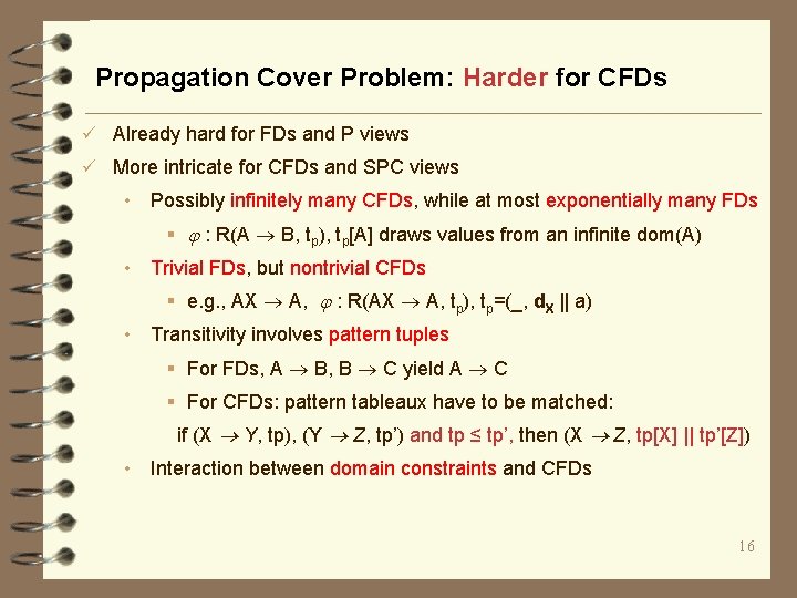
Propagation Cover Problem: Harder for CFDs ü Already hard for FDs and P views ü More intricate for CFDs and SPC views • Possibly infinitely many CFDs, while at most exponentially many FDs § : R(A B, tp), tp[A] draws values from an infinite dom(A) • Trivial FDs, but nontrivial CFDs § e. g. , AX A, : R(AX A, tp), tp=(_, d. X || a) • Transitivity involves pattern tuples § For FDs, A B, B C yield A C § For CFDs: pattern tableaux have to be matched: if (X Y, tp), (Y Z, tp’) and tp ≤ tp’, then (X Z, tp[X] || tp’[Z]) • Interaction between domain constraints and CFDs 16

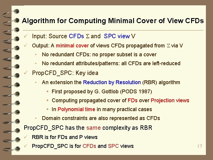
Algorithm for Computing Minimal Cover of View CFDs ü Input: Source CFDs and SPC view V ü Output: A minimal cover of views CFDs propagated from via V • No redundant CFDs: no proper subset is a cover • No redundant attributes/patterns: all CFDs are left-reduced ü Prop. CFD_SPC: Key idea • An extension the Reduction by Resolution (RBR) algorithm § First proposed by G. Gottlob (PODS 1987) § Computing propagated cover of FDs over Projection views § In Polynomial time in many practical cases • Domain constraints are also represented as CFDs Prop. CFD_SPC has the same complexity as RBR ü RBR is for FDs and P views ü Prop. CFD_SPC is for CFDs and SPC views 17

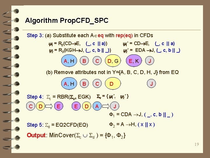
Algorithm Prop. CFD_SPC ü Input R 1 A B R 2 C D E R 3 K G H J • V = ∏Y( F(R 1 R 2 R 3)), where § Y = {A, B, C, D, H, J} § F = {A = H, D = G, E = K } • = { 1, 2}, where § 1 = R 2(CD E, (_, c || a)) § 2 = R 3(KGH J, (_, c, b || _)) ü Step 1: = Min. Cover( ); ü Step 2: (a) EQ = Compute. EQ( F(R 1 R 2 R 3), ) (b) choose representative rep(eq) for each eq class A, H B C D, G E, K J 18

Algorithm Prop. CFD_SPC Step 3: (a) Substitute each A eq with rep(eq) in CFDs 1 = R 2(CD E, (_, c || a)) 2 = R 3(KGH J, (_, c, b || _)) B A, H C 1’ = CD E, (_, c || a) 2’ = EDA J, (_, c, b || _) D, G E, K J (b) Remove attributes not in Y={A, B, C, D, H, J} from EQ B A, H Step 4: c = RBR( v, EGK) C D E E D C D J v = { 1', 2' } A J Ф 1 = CDA J, ( _, c, b || _ ) Step 5: d = EQ 2 CFD(EQ) Ф 2 = A H, ( x || x ) Output: Min. Cover( c d ) = {Ф 1, Ф 2} 19

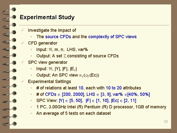
Experimental Study ü Investigate the impact of • The source CFDs and the complexity of SPC views ü CFD generator • Input: , m, n, LHS, var% • Output: A set consisting of source CFDs ü SPC view generator • Input: , |Y|, |F|, |Ec| • Output: An SPC view Y( F(Ec)) ü Experimental Settings • # of relations at least 10, each with 10 to 20 attributes • # of CFDs [200, 2000], LHS [3, 9], var% [40%, 50%] • SPC View: |Y| [5, 50], |F| [1, 10], |Ec| [2, 11] • 1 PC, 3. 00 GHz Intel (R) Pentium (R) D processor, 1 GB of memory • An average of 5 tests on each dataset 20

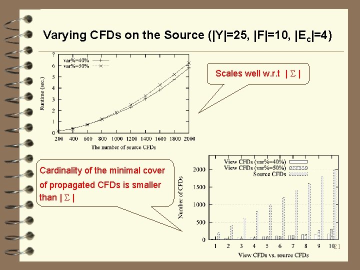
Varying CFDs on the Source (|Y|=25, |F|=10, |Ec|=4) Scales well w. r. t | | Cardinality of the minimal cover of propagated CFDs is smaller than | | 21

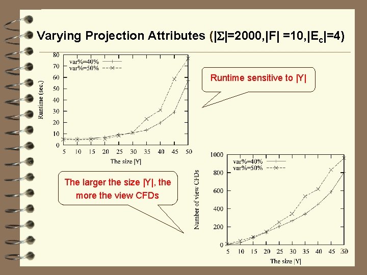
Varying Projection Attributes (| |=2000, |F| =10, |Ec|=4) Runtime sensitive to |Y| The larger the size |Y|, the more the view CFDs 22

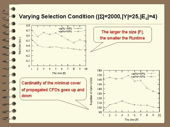
Varying Selection Condition (| |=2000, |Y|=25, |Ec|=4) The larger the size |F|, the smaller the Runtime Cardinality of the minimal cover of propagated CFDs goes up and down 23

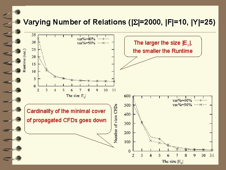
Varying Number of Relations (| |=2000, |F|=10, |Y|=25) The larger the size |Ec|, the smaller the Runtime Cardinality of the minimal cover of propagated CFDs goes down 24

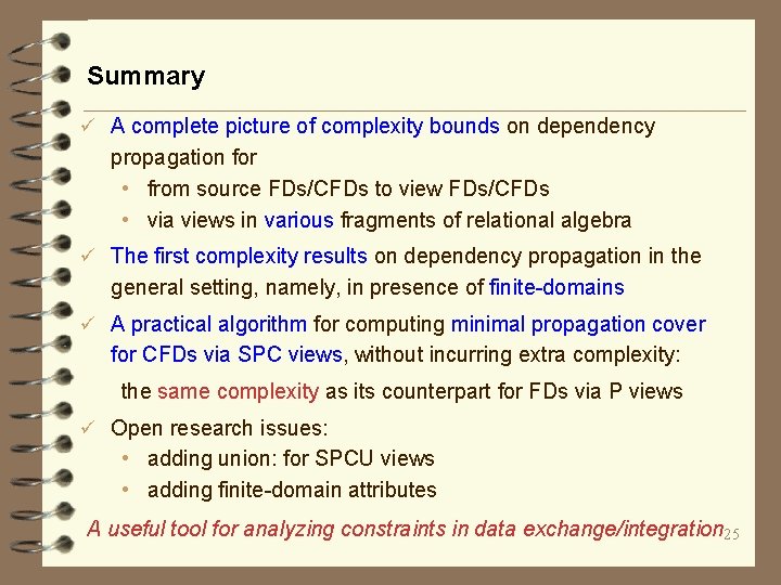
Summary ü A complete picture of complexity bounds on dependency propagation for • from source FDs/CFDs to view FDs/CFDs • via views in various fragments of relational algebra ü The first complexity results on dependency propagation in the general setting, namely, in presence of finite-domains ü A practical algorithm for computing minimal propagation cover for CFDs via SPC views, without incurring extra complexity: the same complexity as its counterpart for FDs via P views ü Open research issues: • adding union: for SPCU views • adding finite-domain attributes A useful tool for analyzing constraints in data exchange/integration 25