Planning the Data Analysis Statistical and Data Processing

Planning the Data Analysis

Statistical and Data Processing Packages 1. Today, in most cases, the computer is used for data processing and analysis. 2. Most students of management are familiar with simple data processing packages like Excel. 3. But for the types and quantum of data generated by a field survey, there is another set of packages available, and the student can choose from several which are commercially available. 4. Some of these packages are: SPSS, SAS, STATISTICA and SYSTAT. There are several others also available, but these four are among the more popular and widely available.

Types of Analysis Packages like SPSS, STATISTICA, etc. can be used for two major types of applications in Research – u Data Processing – General u Statistical Analysis – Specialized (Univariate, Bivariate and Multivariate) Data Processing This application includes coding and entering data for all respondents, for all questions on a questionnaire. For example, there may be a question which asks for the education level of a participant. The choices may be 12 th or below, Graduate, Post-Graduate and any other. The first step in data processing is to assign a code for each of the options – for instance, 1 for 12 th or below, 2 for Graduate, 3 for Post-Graduate and 4 for any other. Next, depending on the option ticked for each respondent, to enter the respective code against his row (usually, the data for one respondent is entered in a row assigned to him in the data set) in the column assigned to the question, in the data matrix.

The end result of data processing for this question would be to be able to tell the researcher how many of the sample of respondents were of education level 12 th or below (Code 1), how many were Graduates (Code 2), how many Post-Graduates (Code 3) and how many were in any other category (Code 4). For example, it could be that out of a sample of 500 respondents, 100 were in Code 1 category, 200 in Code 2, 150 in Code 3, and 50 in Code 4 (Any other). Similarly, all other questions on the questionnaire are processed, and totals for each category of answers can be computed. The menu commands used for such data processing are called FREQUENCIES, SUMMARY STATISTICS, DESCRIPTIVE STATISTICS, or TABLES depending on the software package used.

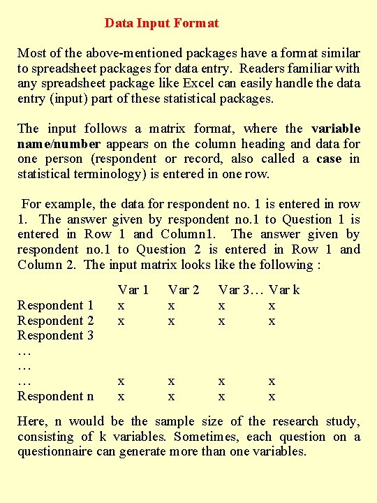
Data Input Format Most of the above-mentioned packages have a format similar to spreadsheet packages for data entry. Readers familiar with any spreadsheet package like Excel can easily handle the data entry (input) part of these statistical packages. The input follows a matrix format, where the variable name/number appears on the column heading and data for one person (respondent or record, also called a case in statistical terminology) is entered in one row. For example, the data for respondent no. 1 is entered in row 1. The answer given by respondent no. 1 to Question 1 is entered in Row 1 and Column 1. The answer given by respondent no. 1 to Question 2 is entered in Row 1 and Column 2. The input matrix looks like the following : Respondent 1 Respondent 2 Respondent 3 … … … Respondent n Var 1 x x Var 2 x x Var 3… Var k x x x Here, n would be the sample size of the research study, consisting of k variables. Sometimes, each question on a questionnaire can generate more than one variables.

Coding One limitation of doing analysis on the computer with these statistical packages is that all data must be converted into numerical form. Otherwise, it cannot be counted or manipulated for analysis. So, all data must be coded and converted to numbers, if it is non-numerical. We saw one example of coding in the previous section, where we gave numerical codes of 1, 2, 3 and 4 to the education level of the respondent. Similarly, any non-numerical data can be converted into numbers. Usually, all nominal scale variables (categorical variables) need to be coded and entered into the packages. An important aspect of coding is to remember which code stands for what. Most software packages have a facility called definition of Value Labels for each variable, which should be used to define the codes for every value of a variable. This is illustrated in a section labelled "value labels" a little later.

Variable Usually, a question on the questionnaire represents a Variable in the package. This is not always the case, because sometimes we may create more than one variables out of answers to a question. For example, it could be a ranking question which requires respondents to rank 5 brands on a scale of 1 to 5. We may define Ranking given to Brand X as variable 10, and ranks given to it could be any number from 1 to 5. Similarly, Ranking of Brand Y could be defined as variable 11, and again, the responses could be from 1 to 5. Therefore, we may end up with 5 variables from that single ranking question on the questionnaire. It all depends on how we want the output to look like, and how we want to analyze it. One very useful provision that all the packages have is the variable name. For instance, if the particular question (variable) represents the respondent’s Income, then the Variable Name can be INCOME on the column representing this variable.

Variable Label and Format There is a provision to give a longer name to each variable if required (usually called Variable Label) in each one of the packages. There is also a provision by which the user can define in these packages the type of variable (Numeric or nonnumeric), and the number of digits it will have. A non-numeric variable can be defined, but no mathematical calculations can be performed with it. For a numerical variable, you can also define the number of decimal points (if applicable). SPSS Commands for Defining Variable Labels In SPSS, you can double click on the column heading of the Variable and fill out the Variable Name, format etc. in the dialog box /table which opens up. In SPSS a table opens up where Variable Name is filled in the first column, and Label in another column, etc.

Value Labels/Codes Sometimes, the different values taken by the variable are continuous numbers. But sometimes, they are categories. For example, income categories could be u. Below 5, 000 per month u 5, 001 to 10, 000 per month u 10, 001 to 20, 000 per month u. More than 20, 000 per month Each of these could be given numerical codes such as 1, 2, 3 or 4. To save these codes along with their meanings (labels) in the computer, we have to use a feature called “Value Labels”. We can use the feature and label 1 as “Below $ 5, 000 p. m. ”, 2 as “$ 5, 001 to 10, 000 p. m. ”, 3 as “$ 10, 001 to 20, 000 p. m. ”, and 4 as “More than $ 20, 000 p. m. ”. The words used in quotes are called Value Labels, and can be defined for each variable separately. For each categorical variable that we have allotted codes to, we need to record the codes along with the Variable Name and Question Number for our records in a separate coding sheet also. Definition of Value Labels simplifies the problems while interpreting the output. The value labels are generally printed along with the codes when a table is printed involving the given variables (for example, income).

Record Number / Case Number Every row is called a “case” or “record”, and represents data for one respondent. If a respondent is represented by one row, usually the row number and the serial number of respondent become identical. In other words, the number of rows will add up to the sample size. If a survey had 100 respondents, 100 rows of data would be entered into the data input matrix.

Missing Data Frequently, respondents do not answer all the questions asked. This leaves some blanks on the questionnaire. There are two approaches for handling this problem. u. Pairwise Deletion : This means that if one respondent’s data is missing for one question, then we simply treat the sample size as one less than the given number of respondents for that question alone, and compute the information asked for. All other questions are treated as usual. u. Listwise Deletion : This means that the results in the entire row of data is deleted, even if there is one missing (blank) piece of data in the questionnaire. This may result in a large reduction in sample size, if there is a lot of missing data on different questions.

Statistical Analysis We have so for discussed general data processing applications of statistical packages. But these packages are capable of a lot of statistical tests, like the chisquared, the ‘t’ test and the ‘F’ test. They can also be used to perform analyses such as Correlation and Regression Analysis, ANOVA or Analysis of Variance, Factor Analysis, Cluster Analysis, Discriminant Analysis, Multidimensional Scaling, Conjoint Analysis and many other advanced statistical analyses. The packages we have mentioned (SPSS, SAS, SYSTAT) generally perform most of these analyses. In addition, the statistical packages also have varying graphical capabilities for drawing graphs.

Approaches to Analysis of data is the process by which data is converted into useful information. Raw data as collected from questionnaires cannot be used unless it is processed in some way to make it amenable to drawing conclusions. Various techniques of data analysis are available, and it is sometimes difficult to choose one that will be the most appropriate for the research problems on hand. The types of analysis to be done and format of output desired should be planned at the time of designing the questionnaire. Three Types of Analysis Broadly, we can classify analysis into three types – 1. Univariate, involving a single variable at a time, 2. Bivariate, involving two variables at a time, and 3. Multivariate, involving three or more variables simultaneously.

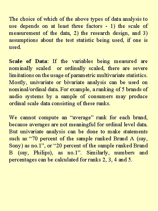
The choice of which of the above types of data analysis to use depends on at least three factors - 1) the scale of measurement of the data, 2) the research design, and 3) assumptions about the test statistic being used, if one is used. Scale of Data: If the variables being measured are nominally scaled or ordinally scaled, there are severe limitations on the usage of parametric multivariate statistics. Mostly, univariate or bivariate analysis can be used on nominal/ordinal data. For example, a ranking of 5 brands of audio systems by a sample of consumers may produce ordinal scale data consisting of these ranks. We cannot compute an “average” rank for each brand, because averages are not meaningful for ordinal level data. But univariate analysis can be done to make statements such as “ 70 percent of the sample ranked Brand A (say, Sony) as no. 1”, or “ 20 percent of the sample ranked Brand B (say, Philips), as no. 1”. Similarly, numbers and percentages can be calculated for ranks 2, 3, 4 and 5.

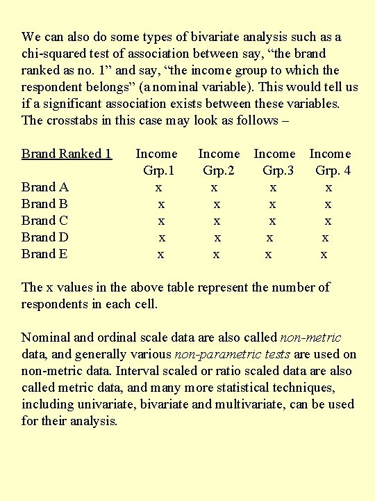
We can also do some types of bivariate analysis such as a chi-squared test of association between say, “the brand ranked as no. 1” and say, “the income group to which the respondent belongs” (a nominal variable). This would tell us if a significant association exists between these variables. The crosstabs in this case may look as follows – Brand Ranked 1 Brand A Brand B Brand C Brand D Brand E Income Grp. 1 x x x Income Grp. 2 x x x Income Grp. 3 x x x Income Grp. 4 x x x The x values in the above table represent the number of respondents in each cell. Nominal and ordinal scale data are also called non-metric data, and generally various non-parametric tests are used on non-metric data. Interval scaled or ratio scaled data are also called metric data, and many more statistical techniques, including univariate, bivariate and multivariate, can be used for their analysis.

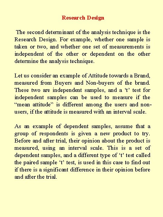
Research Design The second determinant of the analysis technique is the Research Design. For example, whether one sample is taken or two, and whether one set of measurements is independent of the other or dependent on the other determine the analysis technique. Let us consider an example of Attitude towards a Brand, measured from Buyers and Non-buyers of the brand. These two are independent samples, and a ‘t’ test for independent samples can be used to measure if the “mean attitude” is different among the users and nonusers, if the attitude is measured with an interval scale. As an example of dependent samples, assume that a group of respondents is given a new product to try. Before and after trial, their opinion about the product is measured, using an interval scale. This is a set of dependent samples, and a different type of ‘t’ test called the paired sample ‘t’ test, is used in this case to find out if there is a significant difference in their opinion before and after the trial.

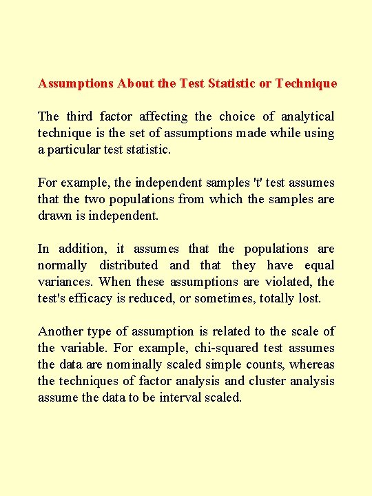
Assumptions About the Test Statistic or Technique The third factor affecting the choice of analytical technique is the set of assumptions made while using a particular test statistic. For example, the independent samples 't' test assumes that the two populations from which the samples are drawn is independent. In addition, it assumes that the populations are normally distributed and that they have equal variances. When these assumptions are violated, the test's efficacy is reduced, or sometimes, totally lost. Another type of assumption is related to the scale of the variable. For example, chi-squared test assumes the data are nominally scaled simple counts, whereas the techniques of factor analysis and cluster analysis assume the data to be interval scaled.

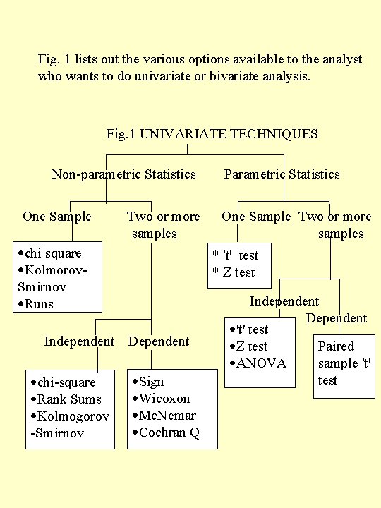
Fig. 1 lists out the various options available to the analyst who wants to do univariate or bivariate analysis. Fig. 1 UNIVARIATE TECHNIQUES Non-parametric Statistics One Sample Two or more samples ·chi square· ·Kolmorov. Smirnov ·Runs Independent ·chi-square ·Rank Sums ·Kolmogorov -Smirnov Parametric Statistics One Sample Two or more samples * 't' test * Z test Dependent ·Sign ·Wicoxon ·Mc. Nemar ·Cochran Q Independent Dependent ·'t' test ·Z test Paired ·ANOVA sample 't' test

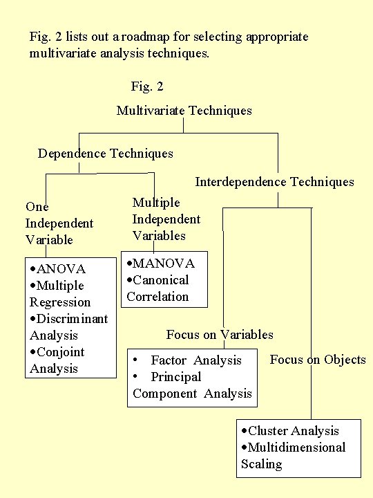
Fig. 2 lists out a roadmap for selecting appropriate multivariate analysis techniques. Fig. 2 Multivariate Techniques Dependence Techniques Interdependence Techniques One Independent Variable ·ANOVA ·Multiple Regression ·Discriminant Analysis ·Conjoint Analysis Multiple Independent Variables ·MANOVA ·Canonical Correlation Focus on Variables • Factor Analysis • Principal Component Analysis Focus on Objects ·Cluster Analysis ·Multidimensional Scaling