Perfect Competition Principles of Economics Shanghai Tech Spring

Perfect Competition Principles of Economics Shanghai. Tech Spring 2018

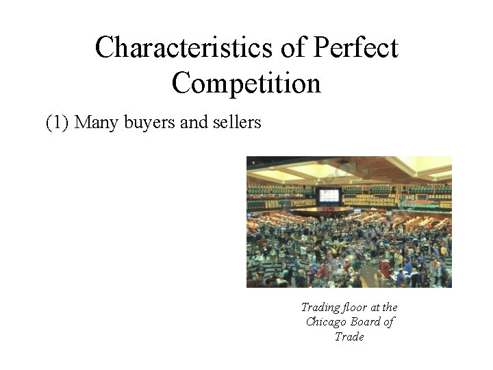
Characteristics of Perfect Competition (1) Many buyers and sellers Trading floor at the Chicago Board of Trade

Characteristics of Perfect Competition (2) Homogeneous products NO BRAND LOYALTY

Characteristics of Perfect Competition (3) No barriers to entry and exit for producers.

EXAMPLES • Barriers to Entry: Patents • Barriers to Exit: High sunk costs

Optimization in the Perfectly Competitive Environment • Firms are PRICE TAKERS • Supply and Demand determine P

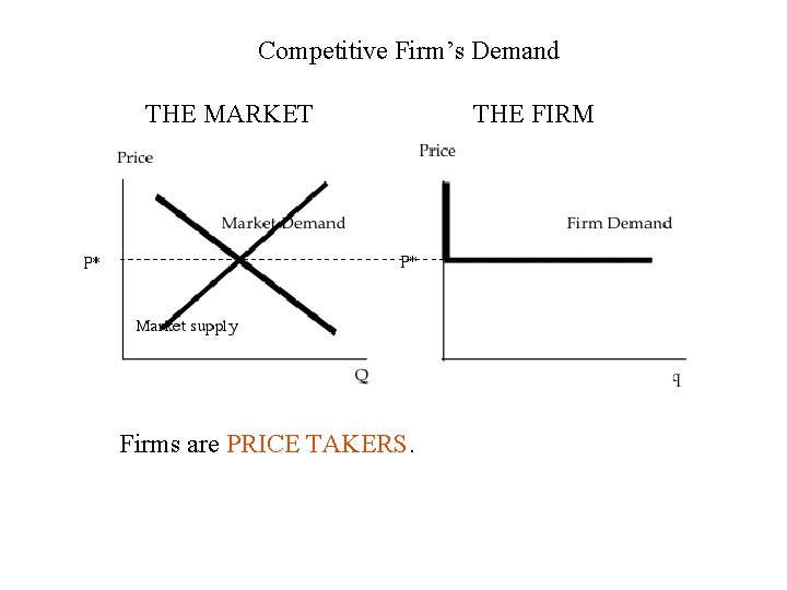
Competitive Firm’s Demand THE MARKET Firms are PRICE TAKERS. THE FIRM

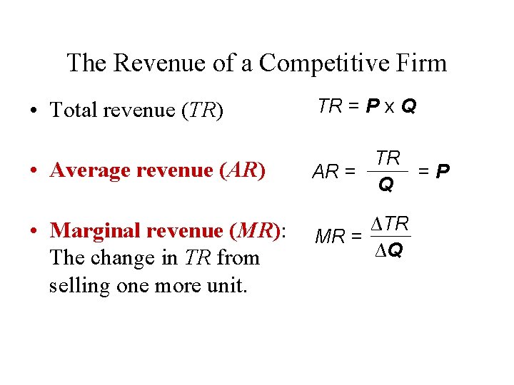
The Revenue of a Competitive Firm • Total revenue (TR) TR = P x Q • Average revenue (AR) TR =P AR = Q • Marginal revenue (MR): The change in TR from selling one more unit. ∆TR MR = ∆Q

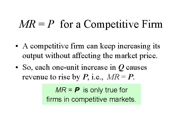
MR = P for a Competitive Firm • A competitive firm can keep increasing its output without affecting the market price. • So, each one-unit increase in Q causes revenue to rise by P, i. e. , MR = P is only true for firms in competitive markets.

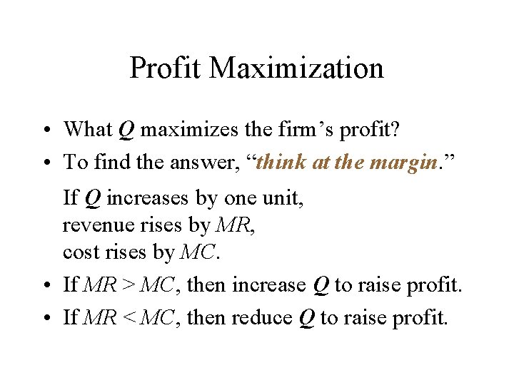
Profit Maximization • What Q maximizes the firm’s profit? • To find the answer, “think at the margin. ” If Q increases by one unit, revenue rises by MR, cost rises by MC. • If MR > MC, then increase Q to raise profit. • If MR < MC, then reduce Q to raise profit.

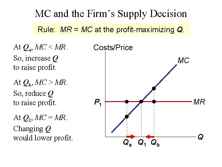
MC and the Firm’s Supply Decision Rule: MR = MC at the profit-maximizing Q. At Qa, MC < MR. So, increase Q to raise profit. At Qb, MC > MR. So, reduce Q to raise profit. At Q 1, MC = MR. Changing Q would lower profit. Costs/Price MC MR P 1 Qa Q 1 Qb Q

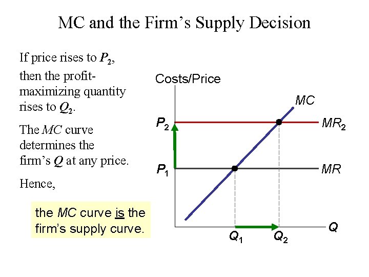
MC and the Firm’s Supply Decision If price rises to P 2, then the profitmaximizing quantity rises to Q 2. The MC curve determines the firm’s Q at any price. Hence, the MC curve is the firm’s supply curve. Costs/Price MC P 2 MR 2 P 1 MR Q 1 Q 2 Q

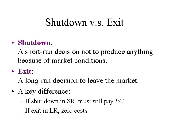
Shutdown v. s. Exit • Shutdown: A short-run decision not to produce anything because of market conditions. • Exit: A long-run decision to leave the market. • A key difference: – If shut down in SR, must still pay FC. – If exit in LR, zero costs.

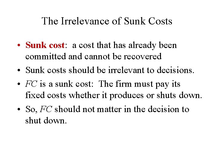
The Irrelevance of Sunk Costs • Sunk cost: a cost that has already been committed and cannot be recovered • Sunk costs should be irrelevant to decisions. • FC is a sunk cost: The firm must pay its fixed costs whether it produces or shuts down. • So, FC should not matter in the decision to shut down.

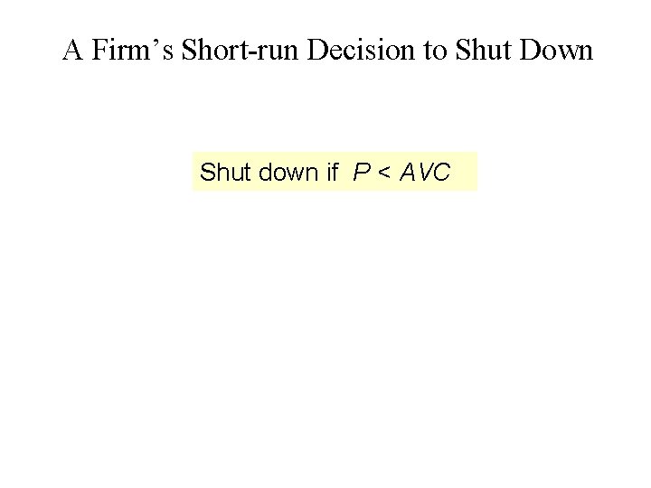
A Firm’s Short-run Decision to Shut Down Shut down if P < AVC

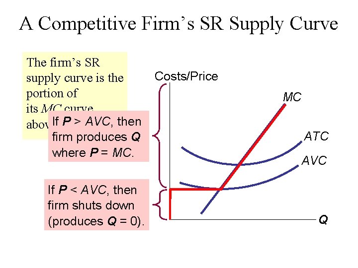
A Competitive Firm’s SR Supply Curve The firm’s SR supply curve is the portion of its MC curve P > AVC, then above. If AVC. firm produces Q where P = MC. If P < AVC, then firm shuts down (produces Q = 0). Costs/Price MC ATC AVC Q

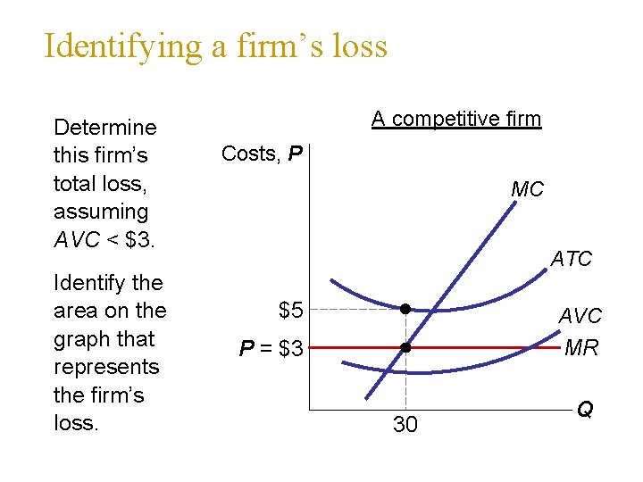
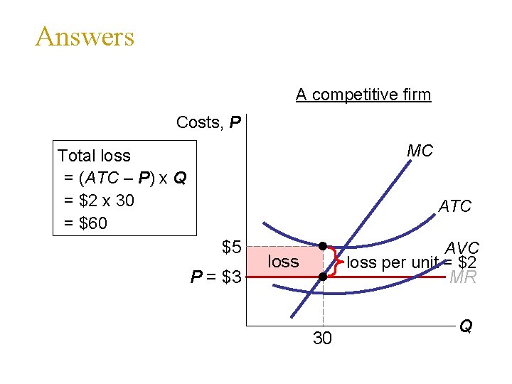
Identifying a firm’s loss Determine this firm’s total loss, assuming AVC < $3. Identify the area on the graph that represents the firm’s loss. A competitive firm Costs, P MC ATC $5 AVC P = $3 MR 30 Q

Answers A competitive firm Costs, P MC Total loss = (ATC – P) x Q = $2 x 30 = $60 ATC $5 P = $3 AVC loss per unit = $2 MR loss 30 Q

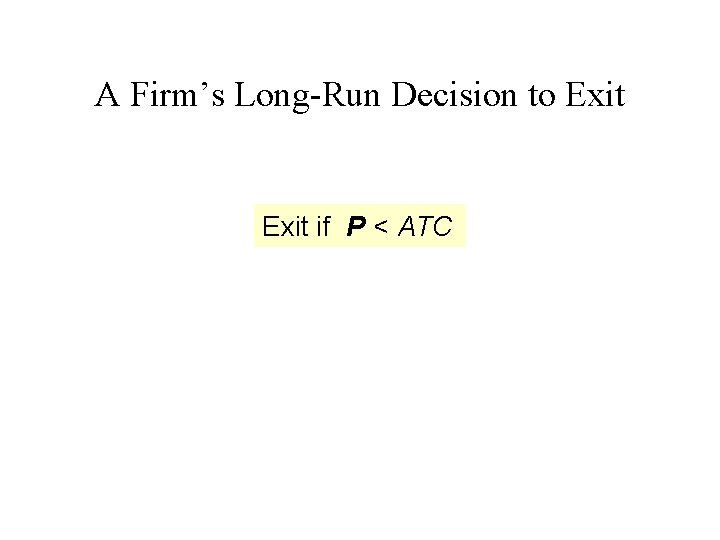
A Firm’s Long-Run Decision to Exit if P < ATC

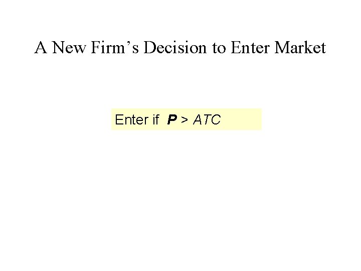
A New Firm’s Decision to Enter Market Enter if P > ATC

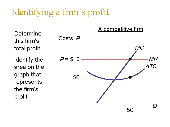
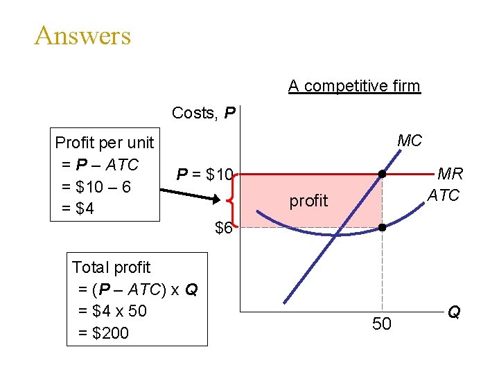
Identifying a firm’s profit Determine this firm’s total profit. Identify the area on the graph that represents the firm’s profit. A competitive firm Costs, P MC MR ATC P = $10 $6 50 Q

Answers A competitive firm Costs, P Profit per unit = P – ATC = $10 – 6 = $4 MC MR ATC P = $10 profit $6 Total profit = (P – ATC) x Q = $4 x 50 = $200 50 Q

Market Supply: Assumptions 1) All existing firms and potential entrants have identical costs. 2) Each firm’s costs do not change as other firms enter or exit the market. 3) The number of firms in the market is – fixed in the short run (due to fixed costs) – variable in the long run (due to free entry and exit)

The SR Market Supply Curve • As long as P ≥ AVC, each firm will produce its profit-maximizing quantity, where MR = MC. • At each price, the market quantity supplied is the sum of quantities supplied by all firms.

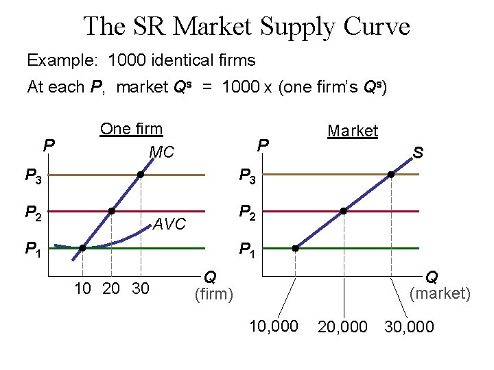
The SR Market Supply Curve Example: 1000 identical firms At each P, market Qs = 1000 x (one firm’s Qs) P One firm MC P P 3 P 2 AVC P 1 Market S P 1 10 20 30 Q (firm) Q (market) 10, 000 20, 000 30, 000

Entry & Exit in the Long Run • In the LR, the number of firms can change due to entry & exit. • If existing firms earn positive economic profit, – new firms enter, SR market supply shifts right. – P falls, reducing profits and slowing entry. • If existing firms incur losses, – some firms exit, SR market supply shifts left. – P rises, reducing remaining firms’ losses.

The Zero-Profit Condition • Long-run equilibrium: The process of entry or exit is complete— remaining firms earn zero economic profit. • In the long run, P = minimum ATC.

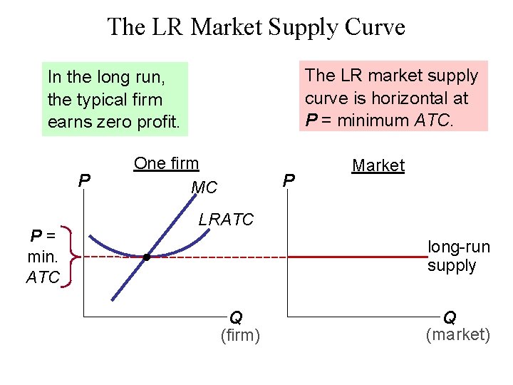
The LR Market Supply Curve The LR market supply curve is horizontal at P = minimum ATC. In the long run, the typical firm earns zero profit. P P= min. ATC One firm MC P Market LRATC long-run supply Q (firm) Q (market)

Why Do Firms Stay in Business if Profit = 0? • Recall, economic profit is revenue minus all costs, including implicit costs like the opportunity cost of the owner’s time and money. • In the zero-profit equilibrium, – firms earn enough revenue to cover these costs – accounting profit is positive

Summary • In competitive markets, managers can only choose quantity, not price • Managers employ marginal reasoning to find q* by equating MR and MC • The Average variable cost curve is used to determine whether losses are great enough to shut down • The individual SR supply curve is MC above its intersection with AVC • In the long run, P = minimum ATC.