Patents and Patent Policy Chapter 23 Patents and

Patents and Patent Policy Chapter 23: Patents and Patent Policy 1

Introduction Information is a public good • Non-rivalry in consumption – If Eli Lilly tells Merck how to make Prozac the information does not leave Lilly – Marginal cost of sharing info, e. g. , the Prozac formula, is zero – Allocationally efficient price = marginal cost = 0 • Non-excludability of people who don’t pay for information – Easy to copy or reverse engineer products – Trade secrets are hard to keep – Effective price is zero • If price of information is zero, no incentive to produce information or develop new products—no dynamic efficiency • Patent Policy must balance the demands of allocational and dynamic efficiency Chapter 23: Patents and Patent Policy 2

Optimal Patent Length • Patents may be used to protect innovators and make the economy more dynamically efficient – Temporarily create monopoly power (bad) – Encourage creation of new products (good) • Two central questions of patent policy – How long should patent last – How wide a range of substitutes should patent span? • Optimal Patent Length – No simple answer such as 14, 17 or 21 years – Nordhaus (1969) classic model illustrates key factors in determining optimal patent length Chapter 23: Patents and Patent Policy 3

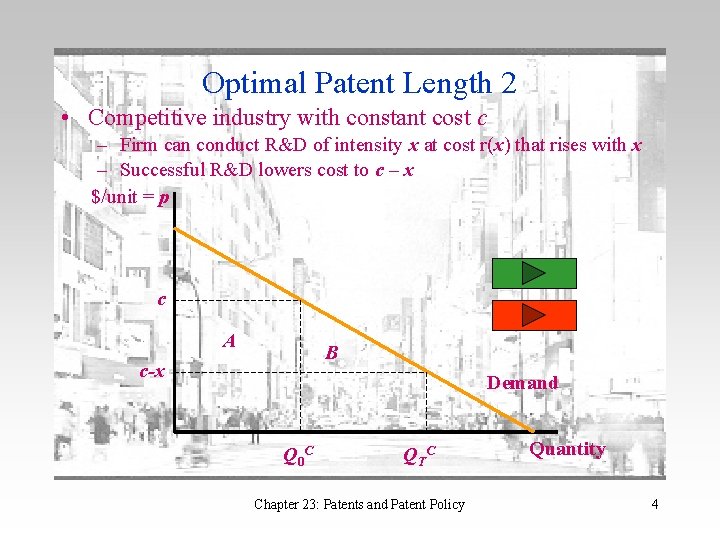
Optimal Patent Length 2 • Competitive industry with constant cost c – Firm can conduct R&D of intensity x at cost r(x) that rises with x – Successful R&D lowers cost to c – x $/unit = p c A B c-x Demand Q 0 C QT C Chapter 23: Patents and Patent Policy Quantity 4

Optimal Patent Length 3 • Assume that patent lasts for T years. – During life of patent, innovator earns monopoly profit area A – When patent expires in T years, consumers gain surplus A plus area B (formerly static deadweight loss) • Trick is to choose length T that gives A to producers for a long enough time to encourage high R&D intensity x and therefore cost savings c – x, incentives to producers but that does not delay the realization of B for too long a time Chapter 23: Patents and Patent Policy 5

Optimal Patent Length 4 • Incentive to producers – – – Size of A research intensity x Present value of A for T year is V(x, T) Cost of research activity is r(x) Net gain of R&D if patent lasts T years is: V(x, T) – r(x) Firms will choose x that maximizes this gain x*(T) Chapter 23: Patents and Patent Policy 6

Optimal Patent Length 5 • Patent Office understands that for any value of T, firms will optimally choose x(T) research intensity – When patent expires in T years, areas A and B are realized as consumer surplus forever. The present value of this surplus that starts in T years is CS(x, T). – Patent policy goal is to maximize net total surplus recognizing that its choice of T determines the amount of R&D intensity x*(T). That is, patent policy aims to maximize: – V[x*(T) , T] – r[x(T)] + CS[x*(T)] – This is a single equation in T and so standard maximization techniques apply Chapter 23: Patents and Patent Policy 7

Optimal Patent Length 6 • Insights of the Nordhaus model 1. Optimal patent length is positive but finite – If T = 0, firms will not do any R&D – As T gets larger § Firms do more R&D § but effect diminishes because the cost of more research intensity r(x) rises & because extra profit in last years of a patent is discounted severely § As T gets larger, society has to wait longer to gain the welfare triangle B. At some point, this cost of dominates the increment to x. T is finite. Chapter 23: Patents and Patent Policy 8

Optimal Patent Length 7 • Insights of the Nordhaus model (cont. ) 2. Optimal patent length is shorter the more elastic is demand – The more elastic demand the greater the static welfare loss B 3. Optimal patent length is shorter the lower the cost of R&D, r(x) – Profit increases linearly with the size of the cost reduction but the welfare loss increases quadratically. – As the equilibrium cost reduction rises, so does the loss from keeping T larger Chapter 23: Patents and Patent Policy 9

Patent Length and Breadth • Optimal patent length may depend on how broad patent protection is – If patents are broad, length should probably be limited because have broad and long patents would confer too much monopoly power – How should policy balance length against breadth of patents? • General Goal: Since the monopoly power of patent will cause welfare loss, choose the design that minimizes the welfare loss per dollar of monopoly profit subject to achieving the profit needed to insure the right innovative effort Chapter 23: Patents and Patent Policy 10

Patent Length and Breadth 2 • Gilbert and Shapiro (1990): Optimal to have very long but narrow patents. Why? – View time as a very long sequence of short-lived intervals – Wish to avoid “jumps” in price—want the marginal value of good to move smoothly so that marginal utility from consumption moves smoothly – When patent expires, price falls to cost which would be a large “jump” – Implication: let patents live long but restrict their breadth so just enough profit is made to do innovation Chapter 23: Patents and Patent Policy 11

Patent Length and Breadth 3 • Klemperer (1990) argues for broad but short-lived patents – Think of products on the Hotelling line—Breadth is fraction of line covered by patent – All ten consumers located at same point as patented product and value it at $10—marginal cost = 0 – If no substitute is available price is $10, no consumer surplus but full surplus of $100 goes to the patented monopolist – What if imperfect substitute is available at cost 0? Chapter 23: Patents and Patent Policy 12

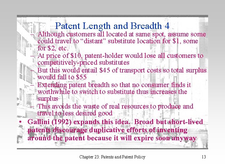
Patent Length and Breadth 4 – Although customers all located at same spot, assume some could travel to “distant” substitute location for $1, some for $2, etc. – At price of $10, patent-holder would lose all customers to competitively-priced substitutes – But this would entail $45 of transport costs so total surplus would fall to $55 – Extending patent breadth so that no consumer finds it worthwhile to switch to substitute thus increases the surplus – This avoids the waste of real resources to produce and travel to less desired good • Gallini (1992) expands this idea. Broad but short-lived patents discourage duplicative efforts of inventing around the patent because it will expire soon anyway Chapter 23: Patents and Patent Policy 13

Patent Length and Breadth 5 • Denicolo (1996) argues that optimal patent length and breadth depends on market conditions— – Long, narrow patents are appropriate for competitive industries – Short, broad patents are appropriate for oligopolistic and monopolistic industries – However, it is hard to implement a policy that doesn’t treat all firms the same. Chapter 23: Patents and Patent Policy 14

Patent Races • Technological break-throughs have a winner-take-all feature—whoever discovers Prozac or invents the Blackberry first wins the patent and associated monopoly power whether they were first by a year or first by a week • This winner-take-all feature makes R&D efforts a bit like a race—all that matters is finishing first • What are the implications of patent races? Chapter 23: Patents and Patent Policy 15

Patent Races 2 • Example: – – Assume two firms, BMI and ECN Developing a new product with Demand: P = 100 – 2 Q. Product will be produced at constant marginal cost c = 50 Development requires a lab and probability of successful development is 0. 8 – Cost of lab is K • Qualitatively, there are three possible outcomes: – Neither firm invests in a lab – One firm invests in a lab and the other doesn’t – Both firms invest in a lab Chapter 23: Patents and Patent Policy 16

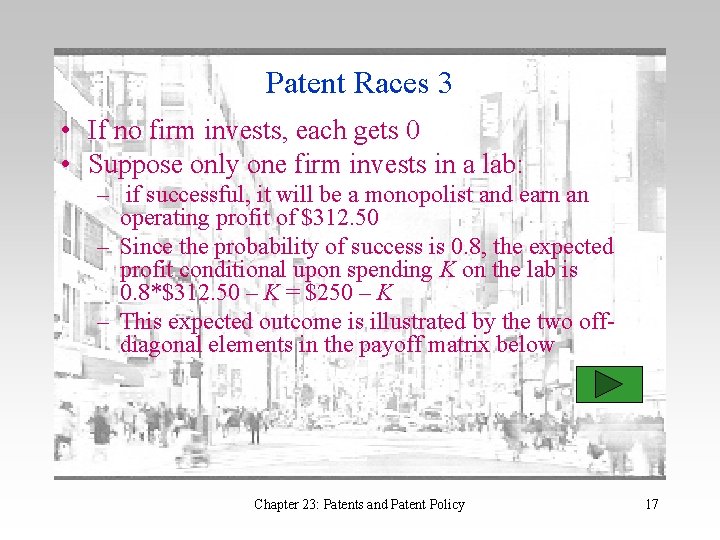
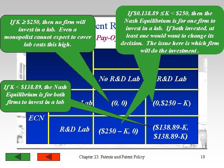
Patent Races 3 • If no firm invests, each gets 0 • Suppose only one firm invests in a lab: – if successful, it will be a monopolist and earn an operating profit of $312. 50 – Since the probability of success is 0. 8, the expected profit conditional upon spending K on the lab is 0. 8*$312. 50 – K = $250 – K – This expected outcome is illustrated by the two offdiagonal elements in the payoff matrix below Chapter 23: Patents and Patent Policy 17

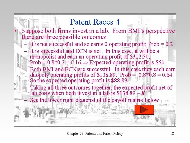
Patent Races 4 • Suppose both firms invest in a lab. From BMI’s perspective there are three possible outcomes – It is not successful and so earns 0 operating profit; Prob = 0. 2 – It is successful and ECN is not. In this case, it will be a monopolist and earn an operating profit of $312. 50; Prob = 0. 8*0. 2 = 0. 16 Expected operating profit is $50. – Both BMI and ECN are successful. In this case they each earn duopoly operating profits of $138. 89. Prob = 0. 8*0. 8 = 0. 64. So the expected operating profit is $88. 89. – Taking all three outcomes together, the expected profit net of lab costs when both invest in a lab is $138. 89 – K – See the lower right diagonal of the payoff matrix below Chapter 23: Patents and Patent Policy 18

If $0. 138. 89 K < $250, then the Nash Equilibrium is for one firm to If K $250, then no firm will invest in a lab. If both invested, at invest in a lab. Even a least one would want to change its monopolist cannot expect to cover The Pay-Off Matrix decision. The issue here is which firm lab costs this high. will do the investment. Patent Races 5 BMI If K < $138. 89, the Nash Equilibrium is for both firms to invest in No a lab. R&D Lab No R&D Lab (0, 0) (0, $250 – K) ($250 – K, 0) ($138. 89 -K, $138. 89 -K) ECN R&D Lab Chapter 23: Patents and Patent Policy 19

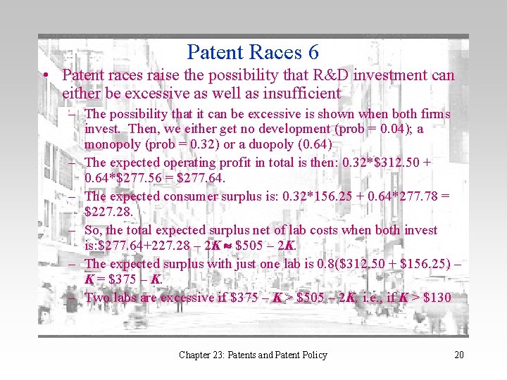
Patent Races 6 • Patent races raise the possibility that R&D investment can either be excessive as well as insufficient – The possibility that it can be excessive is shown when both firms invest. Then, we either get no development (prob = 0. 04); a monopoly (prob = 0. 32) or a duopoly (0. 64) – The expected operating profit in total is then: 0. 32*$312. 50 + 0. 64*$277. 56 = $277. 64. – The expected consumer surplus is: 0. 32*156. 25 + 0. 64*277. 78 = $227. 28. – So, the total expected surplus net of lab costs when both invest is: $277. 64+227. 28 – 2 K $505 – 2 K. – The expected surplus with just one lab is 0. 8($312. 50 + $156. 25) – K = $375 – K. – Two labs are excessive if $375 – K > $505 – 2 K, i. e. , if K > $130 Chapter 23: Patents and Patent Policy 20

Patent Races 7 • The reason that R&D can be excessive is wasteful duplication. Each firm thinks only about its own potential gain and not about the fact that if both are successful (which is fairly likely given that the probability of a successful lab is 0. 8) they will hurt each other’s profit • However, there can also be too little investment. • This is because firms do not consider the increased consumer surplus that successful development of a new product will generate Chapter 23: Patents and Patent Policy 21

“Sleeping” Patents • Most firms have many patents including some that they never use. Similarly, many film studios buy the rights to books and plays but never produce them. • Instead, these patents and copyrights are left dormant or sleeping. Why? • The answer is that it is worth more to the incumbent monopolist to make sure that a rival does not enter than it is for the rival to acquire the patent or copyright and come in as a duopolist. Chapter 23: Patents and Patent Policy 22

“Sleeping” Patents 2 • Consider a market with demand: P = 100 – Q. – An incumbent monopolist with constant unit cost c. I = $20 based on the firm’s unique technology – There is an alternative technology with constant cost c. A = $30 • Monopolist has a patent on the alternative process. It can sell it to its rival or let it sleep. Which will it do? – At existing low cost [c. I = $20] technology, monopolist sets price of $60, sells 40 units and earns profit of $1, 600 Chapter 23: Patents and Patent Policy 23

“Sleeping” Patents 3 • Suppose competition is Bertrand: – If rival has patent and ability to produce at c. A = $30, rival will earn no profit because it can’t compete with c. I = $20 – But rival’s presence will constrain monopolist to set P no higher than $30—Profit will fall to $700 • CONCLUSION: – If competition is Bertrand, the rival will not pay anything for it and it is worth $1, 600 - $700 = $900 to the monopolist – Monopolist will let the alternative technology patent sleep Chapter 23: Patents and Patent Policy 24

Sleeping Patents 4 • What if competition is Cournot? – Incumbent has cost c. I = $20; Rival has cost c. A = $30 – Duopoly outcome is: • Incumbent output is 30; Rival output is 20 • Incumbent profit is $900; Rival profit is $400 – If rival has access to the alternative technology, incumbent loses $1600 – $900 = $700 in profit – Most rival gains is $400 • CONCLUSION: – Again, it is worth more to the incumbent to keep the patent on the alternative technology sleeping than it is to the rival to buy it out Chapter 23: Patents and Patent Policy 25

Patent Licensing • Incumbents will often prevent rival entrant access to alternative, high cost technology and keep it sleeping. • But firms may license the best, low-cost technology • Why? There is a difference between keeping new firms out versus competing with existing rivals. • The profitability of licensing depends on – Nature of competition – Drastic versus non-drastic innovation Chapter 23: Patents and Patent Policy 26

Patent Licensing 2 • Consider previous example with demand: P = 100 – Q – Imagine that we now start with 2 firms each with constant marginal cost of c. A = $30 – The Cournot equilibrium results in each firm producing 23. 33 units • Total Output is Q = 46. 67 • Price is P = $53. 333 • Profit to each firm is $272. 222 Chapter 23: Patents and Patent Policy 27

Patent Licensing 3 • Let one firm develop new technology with cost c. I = $20 – The new equilibrium has P = $50 – Low-cost firm produces 30 units; earns profit of $900 – High cost firms produces 20 units; earns profit of $400 • What happens if low cost firm licenses its technology to high cost firm for a fee of (just under) $10 per unit. – Market outcome is unchanged from the original equilibrium. – High cost firm now produce at $20 per unit but also has to pay (nearly) $10 in licensing fees. – Effectively, the high-cost firm still has a unit cost of $30 – Low cost firm still earns $900 profit from production, BUT § It also picks up $10*20 = $200 in licensing fees § Licensing definitely pays off Chapter 23: Patents and Patent Policy 28

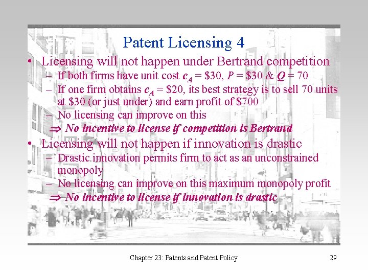
Patent Licensing 4 • Licensing will not happen under Bertrand competition – If both firms have unit cost c. A = $30, P = $30 & Q = 70 – If one firm obtains c. A = $20, its best strategy is to sell 70 units at $30 (or just under) and earn profit of $700 – No licensing can improve on this No incentive to license if competition is Bertrand • Licensing will not happen if innovation is drastic – Drastic innovation permits firm to act as an unconstrained monopoly – No licensing can improve on this maximum monopoly profit No incentive to license if innovation is drastic Chapter 23: Patents and Patent Policy 29

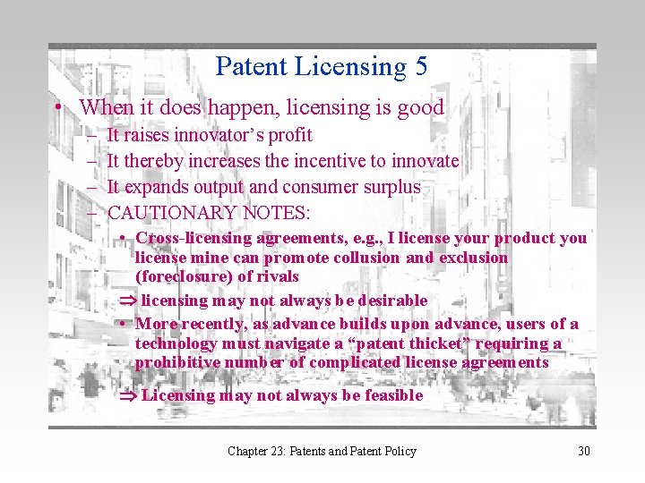
Patent Licensing 5 • When it does happen, licensing is good – – It raises innovator’s profit It thereby increases the incentive to innovate It expands output and consumer surplus CAUTIONARY NOTES: • Cross-licensing agreements, e. g. , I license your product you license mine can promote collusion and exclusion (foreclosure) of rivals licensing may not always be desirable • More recently, as advance builds upon advance, users of a technology must navigate a “patent thicket” requiring a prohibitive number of complicated license agreements Licensing may not always be feasible Chapter 23: Patents and Patent Policy 30

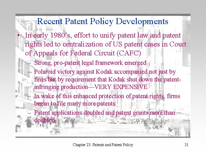
Recent Patent Policy Developments • In early 1980’s, effort to unify patent law and patent rights led to centralization of US patent cases in Court of Appeals for Federal Circuit (CAFC) – Strong, pro-patent legal framework emerged – Polaroid victory against Kodak accompanied not just by fines but by requirement that Kodak shut down the patentinfringing production—VERY EXPENSIVE – In wake of this enhanced protection of patent rights, firms began to file many more patents – Patent applications doubled and patent grants more than doubled Chapter 23: Patents and Patent Policy 31

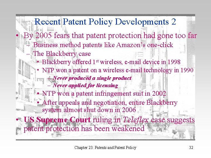
Recent Patent Policy Developments 2 • By 2005 fears that patent protection had gone too far – Business method patents like Amazon’s one-click – The Blackberry case • Blackberry offered 1 st wireless, e-mail device in 1998 • NTP won a patent on a wireless e-mail technology in 1990 – Never produced a single product – Never applied for licensing • NTP won a patent infringement suit in 2002 • After appeals and negotiation, entire Blackberry system almost shut down in 2006 • US Supreme Court ruling in Teleflex case suggests patent protection has been weakened Chapter 23: Patents and Patent Policy 32

Empirical Application: Patent Explosion in US Semiconductor Industry • Patent awards per million $ of R&D doubled in the US semiconductor industry in decade after CAFC emerged as main patent court • Why this increase? – New patent law environment – Or something else • Need a model of patent process – Think of number of patents p in a given time period as a random variable – What random process makes sense? Chapter 23: Patents and Patent Policy 33

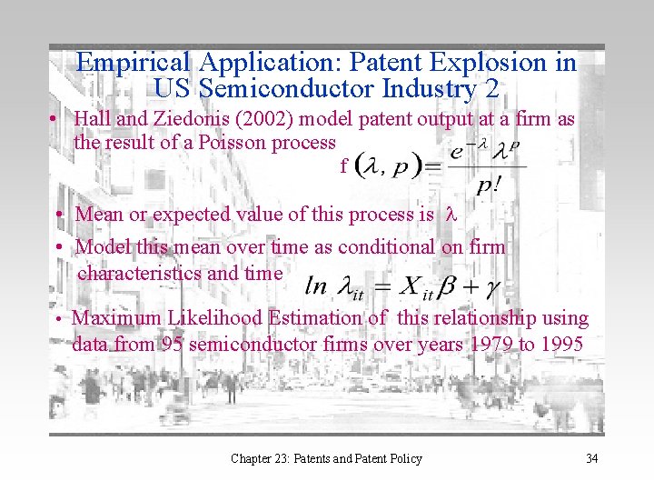
Empirical Application: Patent Explosion in US Semiconductor Industry 2 • Hall and Ziedonis (2002) model patent output at a firm as the result of a Poisson process f • Mean or expected value of this process is • Model this mean over time as conditional on firm characteristics and time • Maximum Likelihood Estimation of this relationship using data from 95 semiconductor firms over years 1979 to 1995 Chapter 23: Patents and Patent Policy 34

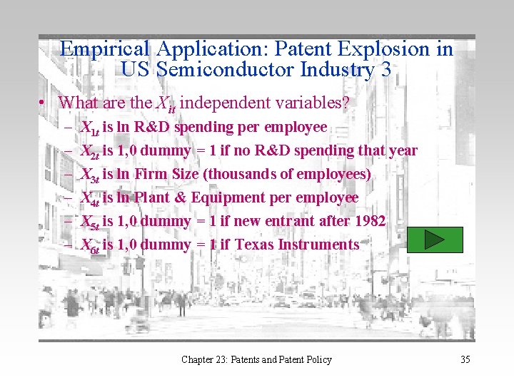
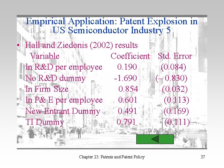
Empirical Application: Patent Explosion in US Semiconductor Industry 3 • What are the Xit independent variables? – – – X 1 t is ln R&D spending per employee X 2 t is 1, 0 dummy = 1 if no R&D spending that year X 3 t is ln Firm Size (thousands of employees) X 4 t is ln Plant & Equipment per employee X 5 t is 1, 0 dummy = 1 if new entrant after 1982 X 6 t is 1, 0 dummy = 1 if Texas Instruments Chapter 23: Patents and Patent Policy 35

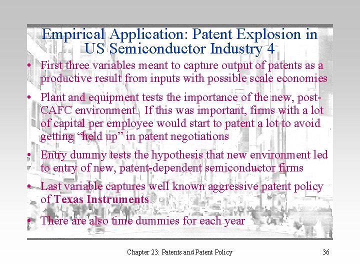
Empirical Application: Patent Explosion in US Semiconductor Industry 4 • First three variables meant to capture output of patents as a productive result from inputs with possible scale economies • Plant and equipment tests the importance of the new, post. CAFC environment. If this was important, firms with a lot of capital per employee would start to patent a lot to avoid getting “held up” in patent negotiations • Entry dummy tests the hypothesis that new environment led to entry of new, patent-dependent semiconductor firms • Last variable captures well known aggressive patent policy of Texas Instruments • There also time dummies for each year Chapter 23: Patents and Patent Policy 36

Empirical Application: Patent Explosion in US Semiconductor Industry 5 • Hall and Ziedonis (2002) results Variable Coefficient Std. Error ln R&D per employee 0. 190 (0. 084) No R&D dummy -1. 690 (– 0. 830) ln Firm Size 0. 854 (0. 032) ln P& E per employee 0. 601 (0. 113) New Entrant Dummy 0. 491 (0. 169) TI Dummy 0. 791 (0. 111) Chapter 23: Patents and Patent Policy 37

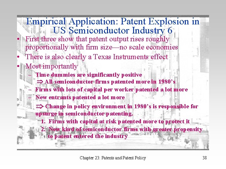
Empirical Application: Patent Explosion in US Semiconductor Industry 6 • First three show that patent output rises roughly proportionally with firm size—no scale economies • There is also clearly a Texas Instruments effect • Most importantly – Time dummies are significantly positive All semiconductor firms patented more in 1980’s – Firms with lots of capital per worker patented a lot more – New entrants patented a lot more Change in policy environment in 1980’s is responsible for upsurge in semiconductor patenting. 1. Firms with capital at risk patented more to protect it 2. New kind of semiconductor firms with greater propensity to patent entered the industry Chapter 23: Patents and Patent Policy 38