Patents and Patent Policy Chapter 23 Patents and

Patents and Patent Policy Chapter 23: Patents and Patent Policy 1

Introduction Information is a public good • Non-rivalry in consumption – If Eli Lilly tells Merck how to make Prozac the information does not leave Lilly – Marginal cost of sharing info, e. g. , the Prozac formula, is zero – Allocationally efficient price = marginal cost = 0 • Non-excludability of people who don’t pay for information – Easy to copy or reverse engineer products – Trade secrets are hard to keep – Effective price is zero • If price of information is zero, no incentive to produce information or develop new products—no dynamic efficiency • Patent Policy must balance the demands of allocational and dynamic efficiency Chapter 23: Patents and Patent Policy 2

Optimal Patent Length Patents may be used to protect innovators and make the economy more dynamically efficient • Temporarily create monopoly power (bad) • Encourage creation of new products (good) Two central questions of patent policy • How long should patent last • How wide a range of substitutes should patent span? Optimal Patent Length • No simple answer such as 14, 17 or 21 years • Nordhaus (1969) classic model illustrates key factors in determining optimal patent length Chapter 23: Patents and Patent Policy 3

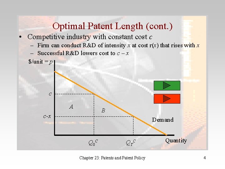
Optimal Patent Length (cont. ) • Competitive industry with constant cost c – Firm can conduct R&D of intensity x at cost r(x) that rises with x – Successful R&D lowers cost to c – x $/unit = p c A B c-x Demand Q 0 C QT C Chapter 23: Patents and Patent Policy Quantity 4

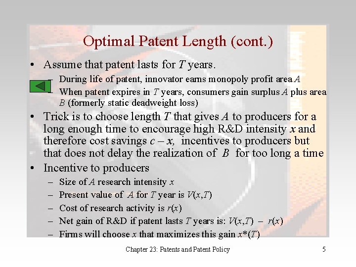
Optimal Patent Length (cont. ) • Assume that patent lasts for T years. – During life of patent, innovator earns monopoly profit area A – When patent expires in T years, consumers gain surplus A plus area B (formerly static deadweight loss) • Trick is to choose length T that gives A to producers for a long enough time to encourage high R&D intensity x and therefore cost savings c – x, incentives to producers but that does not delay the realization of B for too long a time • Incentive to producers – – – Size of A research intensity x Present value of A for T year is V(x, T) Cost of research activity is r(x) Net gain of R&D if patent lasts T years is: V(x, T) – r(x) Firms will choose x that maximizes this gain x*(T) Chapter 23: Patents and Patent Policy 5

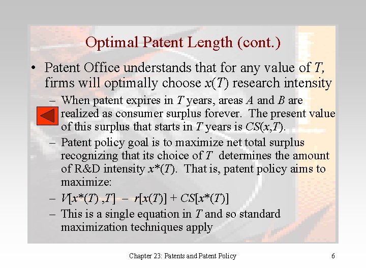
Optimal Patent Length (cont. ) • Patent Office understands that for any value of T, firms will optimally choose x(T) research intensity – When patent expires in T years, areas A and B are realized as consumer surplus forever. The present value of this surplus that starts in T years is CS(x, T). – Patent policy goal is to maximize net total surplus recognizing that its choice of T determines the amount of R&D intensity x*(T). That is, patent policy aims to maximize: – V[x*(T) , T] – r[x(T)] + CS[x*(T)] – This is a single equation in T and so standard maximization techniques apply Chapter 23: Patents and Patent Policy 6

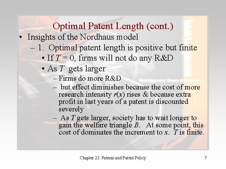
Optimal Patent Length (cont. ) • Insights of the Nordhaus model – 1. Optimal patent length is positive but finite • If T = 0, firms will not do any R&D • As T gets larger – Firms do more R&D – but effect diminishes because the cost of more research intensity r(x) rises & because extra profit in last years of a patent is discounted severely – As T gets larger, society has to wait longer to gain the welfare triangle B. At some point, this cost of dominates the increment to x. T is finite. Chapter 23: Patents and Patent Policy 7

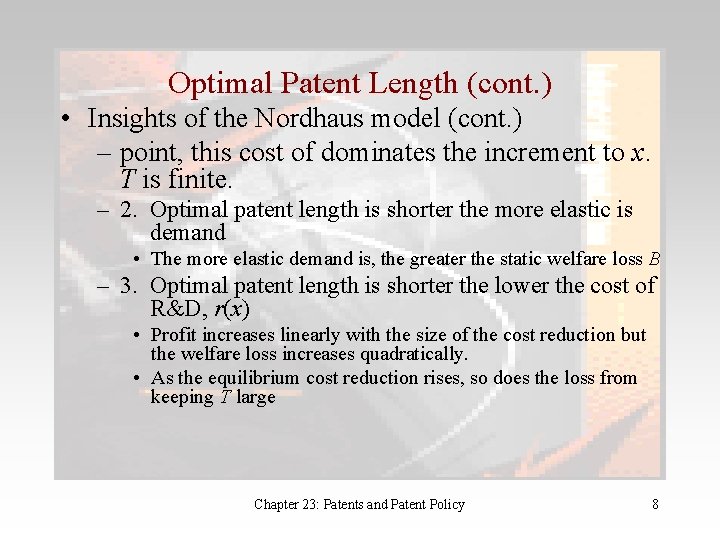
Optimal Patent Length (cont. ) • Insights of the Nordhaus model (cont. ) – point, this cost of dominates the increment to x. T is finite. – 2. Optimal patent length is shorter the more elastic is demand • The more elastic demand is, the greater the static welfare loss B – 3. Optimal patent length is shorter the lower the cost of R&D, r(x) • Profit increases linearly with the size of the cost reduction but the welfare loss increases quadratically. • As the equilibrium cost reduction rises, so does the loss from keeping T large Chapter 23: Patents and Patent Policy 8

Patent Length and Breadth • Optimal patent length may depend on how broad patent protection is – If patents are broad, length should probably be limited because have broad and long patents would confer too much monopoly power – Broad patent protection has the advantage that it prevents minor alterations on the original invention [Klemperer (1990)] – Long patents may actually discourage innovation [Gallini (1992)]. • With short patents, rivals can afford to wait until patent expires • If patents are long, rivals cannot wait but will try to invent around the patent. The anticipation of this copycat activity may depress innovation – Denicolo (1996) argues that optimal patent length and breadth depends on market conditions—The more competitive an industry the more long, narrow patents are desirable – Unfortunately, while the Denicolo argument may be rational, it is hard to implement a policy that doesn’t treat all firms the same. Chapter 23: Patents and Patent Policy 9

Patent Races • Technological break-throughs have a winner-take-all feature—whoever discovers Prozac or invents a new good wins the patent and associated monopoly power whether they were first by a year or first by a week • This winner-take-all feature makes R&D efforts a bit like a race—all that matters is finishing first • What are the implications of patent races? • Example: – – Assume two firms, BMI and ECN Developing a new product for which Demand is P = 100 – 2 Q. Product will be produced at constant marginal cost c = 50 Development requires a lab and probability of successful development is 0. 8 – Cost of lab is K Chapter 23: Patents and Patent Policy 10

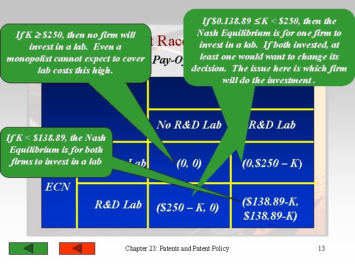
Patent Races (cont. ) • Qualitatively, there are three possible outcomes: – Neither firm invests in a lab – One firm invests in a lab and the other doesn’t – Both firms invest in a lab • If no firm invests, each gets 0 • Suppose only one firm invests in a lab: – if successful, it will be a monopolist and earn an operating profit of $312. 50 – Since the probability of success is 0. 8, the expected profit conditional upon spending K on the lab is 0. 8*$312. 50 – K = $250 – K – This expected outcome is illustrated by the two offdiagonal elements in the payoff matrix below Chapter 23: Patents and Patent Policy 11

Patent Races (cont. ) • Suppose both firms invest in a lab. From BMI’s perspective there are three possible outcomes – It is not successful and so earns 0 operating profit. This happens with probability 0. 2 – It is successful and ECN is not. In this case, it will be a monopolist and earn an operating profit of $312. 50. This happens with probability, 0. 8*0. 2 = 0. 16. The expected operating profit is therefore $50. – Both BMI and ECN are successful. In this case they each earn duopoly operating profits of $138. 89. This happens with probability, 0. 8*0. 8 = 0. 64. So the expected operating profit is $88. 89. – Taking all three outcomes together, the expected profit net of lab costs when both invest in a lab is $138. 89 – K – This is shown in the lower right diagonal of the payoff matrix below Chapter 23: Patents and Patent Policy 12

If $0. 138. 89 K < $250, then the Nash Equilibrium is for one firm to If K $250, then no firm will invest in a lab. If both invested, at invest in a lab. Even a least one would want to change its monopolist cannot expect to cover The Pay-Off Matrix decision. The issue here is which firm lab costs this high. will do the investment. Patent Races (cont. ) BMI If K < $138. 89, the Nash Equilibrium is for both firms to invest in No a lab. R&D Lab No R&D Lab (0, 0) (0, $250 – K) ($250 – K, 0) ($138. 89 -K, $138. 89 -K) ECN R&D Lab Chapter 23: Patents and Patent Policy 13

Patent Races (cont. ) • Patent races raise the possibility that R&D investment can either be excessive or insufficient – The possibility that it can be excessive is illustrated by the outcome in which both firms invest. When both invest, we either get no development (prob = 0. 04); a monopoly (prob = 0. 32) or a duopoly (0. 64) – The expected operating profit in total is then: 0. 32*$312. 50 + 0. 64*$277. 56 = $277. 64. – The expected consumer surplus is: 0. 32*156. 25 + 0. 64*277. 78 = $227. 28. – So, the total expected surplus net of lab costs when both invest is: $277. 64+227. 28 – 2 K $505 – 2 K. – The expected surplus with just one lab is 0. 8($312. 50 + $156. 25) – K = $375 – K. – Two labs are excessive if $375 – K > $505 – 2 K, I. e. , if K > $130 Chapter 23: Patents and Patent Policy 14

Patent Races (cont. ) • The reason that R&D can be excessive is wasteful duplication. Each firm thinks only about its own potential gain and not about the fact that if both are successful (which is fairly likely given that the probability of a successful lab is 0. 8) they will hurt each other’s profit • However, there can also be too little investment. • This is because firms do not consider the increased consumer surplus that successful development of a new product will generate Chapter 23: Patents and Patent Policy 15

“Sleeping” Patents • Most firms have many patents including some that they never use. Similarly, many film studios buy the rights to books and plays but never produce them. • Instead, these patents and copyrights are left dormant or sleeping. Why? • The answer is that it is worth more to the incumbent monopolist to make sure that a rival does not enter than it is for the rival to acquire the patent or copyright and come in as a duopolist. • Consider a market with demand: P = 100 – Q. – An incumbent monopolist with constant unit cost c. I = $20 based on the firm’s unique technology – There is an alternative technology with constant cost c. A = $30 Chapter 23: Patents and Patent Policy 16

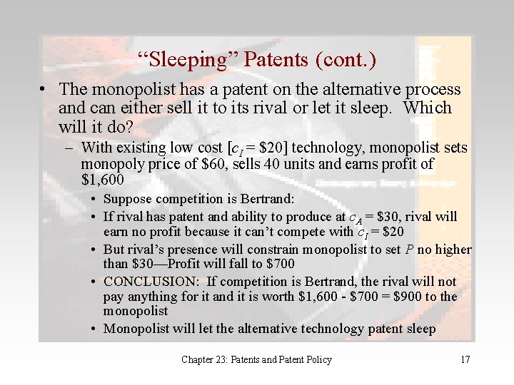
“Sleeping” Patents (cont. ) • The monopolist has a patent on the alternative process and can either sell it to its rival or let it sleep. Which will it do? – With existing low cost [c. I = $20] technology, monopolist sets monopoly price of $60, sells 40 units and earns profit of $1, 600 • Suppose competition is Bertrand: • If rival has patent and ability to produce at c. A = $30, rival will earn no profit because it can’t compete with c. I = $20 • But rival’s presence will constrain monopolist to set P no higher than $30—Profit will fall to $700 • CONCLUSION: If competition is Bertrand, the rival will not pay anything for it and it is worth $1, 600 - $700 = $900 to the monopolist • Monopolist will let the alternative technology patent sleep Chapter 23: Patents and Patent Policy 17

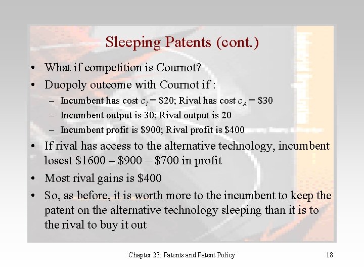
Sleeping Patents (cont. ) • What if competition is Cournot? • Duopoly outcome with Cournot if : – Incumbent has cost c. I = $20; Rival has cost c. A = $30 – Incumbent output is 30; Rival output is 20 – Incumbent profit is $900; Rival profit is $400 • If rival has access to the alternative technology, incumbent losest $1600 – $900 = $700 in profit • Most rival gains is $400 • So, as before, it is worth more to the incumbent to keep the patent on the alternative technology sleeping than it is to the rival to buy it out Chapter 23: Patents and Patent Policy 18

Patent Licensing • Incumbents will prevent rival entrant access to alternative, high cost technology and keep it sleeping. • But firms may license the best, low-cost technology • Why? There is a difference between keeping new firms out versus competing with existing rivals. • The profitability of licensing depends on – Nature of competition – Drastic versus non-drastic innovation Chapter 23: Patents and Patent Policy 19

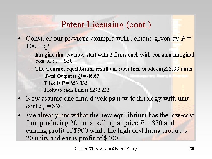
Patent Licensing (cont. ) • Consider our previous example with demand given by P = 100 – Q – Imagine that we now start with 2 firms each with constant marginal cost of c. A = $30 – The Cournot equilibrium results in each firm producing 23. 33 units • Total Output is Q = 46. 67 • Price is P = $53. 333 • Profit to each firm is $272. 222 • Now assume one firm develops new technology with unit cost c. I = $20 • We already know that the new equilibrium has the low-cost firm producing 30 units, selling at price P = $50 and earning profit of $900 while the high cost firms produces 20 units and earns profit of $400 Chapter 23: Patents and Patent Policy 20

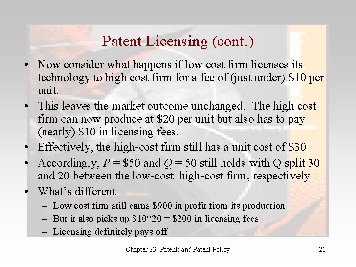
Patent Licensing (cont. ) • Now consider what happens if low cost firm licenses its technology to high cost firm for a fee of (just under) $10 per unit. • This leaves the market outcome unchanged. The high cost firm can now produce at $20 per unit but also has to pay (nearly) $10 in licensing fees. • Effectively, the high-cost firm still has a unit cost of $30 • Accordingly, P = $50 and Q = 50 still holds with Q split 30 and 20 between the low-cost high-cost firm, respectively • What’s different – Low cost firm still earns $900 in profit from its production – But it also picks up $10*20 = $200 in licensing fees – Licensing definitely pays off Chapter 23: Patents and Patent Policy 21

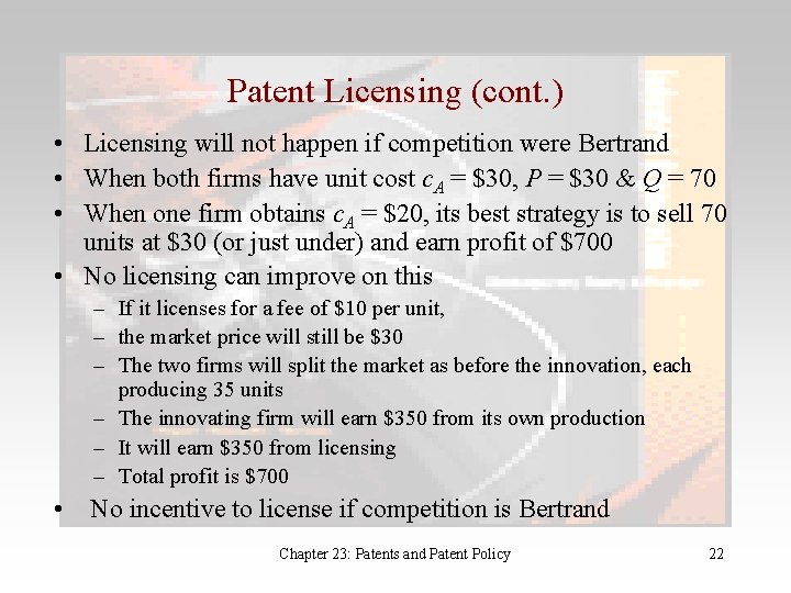
Patent Licensing (cont. ) • Licensing will not happen if competition were Bertrand • When both firms have unit cost c. A = $30, P = $30 & Q = 70 • When one firm obtains c. A = $20, its best strategy is to sell 70 units at $30 (or just under) and earn profit of $700 • No licensing can improve on this – If it licenses for a fee of $10 per unit, – the market price will still be $30 – The two firms will split the market as before the innovation, each producing 35 units – The innovating firm will earn $350 from its own production – It will earn $350 from licensing – Total profit is $700 • No incentive to license if competition is Bertrand Chapter 23: Patents and Patent Policy 22

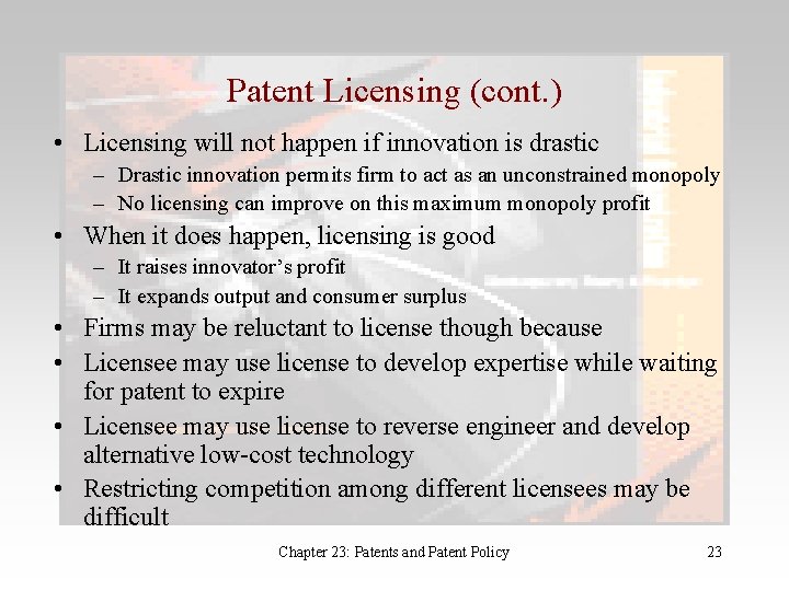
Patent Licensing (cont. ) • Licensing will not happen if innovation is drastic – Drastic innovation permits firm to act as an unconstrained monopoly – No licensing can improve on this maximum monopoly profit • When it does happen, licensing is good – It raises innovator’s profit – It expands output and consumer surplus • Firms may be reluctant to license though because • Licensee may use license to develop expertise while waiting for patent to expire • Licensee may use license to reverse engineer and develop alternative low-cost technology • Restricting competition among different licensees may be difficult Chapter 23: Patents and Patent Policy 23