OVERVIEW APPLICATION OF HAWKES PROCESS Dr Soumaya Mauthoor

OVERVIEW & APPLICATION OF HAWKES PROCESS Dr Soumaya Mauthoor Mar 2019

2002 • Physics MSc 2006 • Physics Ph. D 2011 • Data Consultant 2016 • Operations Researcher 2017 • Data Scientist • MData. Gov

Outline MOTIVATION HAWKES PROCESS INFERENCE AND DIAGNOSTICS EXTENSIONS SEISMIC ACTIVITY CRIME EPIDEMICS CAUTION

Motivation These 4 processes exhibit self-excitation: The occurrence of events promotes future events. As an analyst, we want to find out: • Does the rate of events vary in space and time? • What spatial or temporal covariates may be related to the rate of events? • What is the triggering rate? • How are the triggered events distributed in space and time?

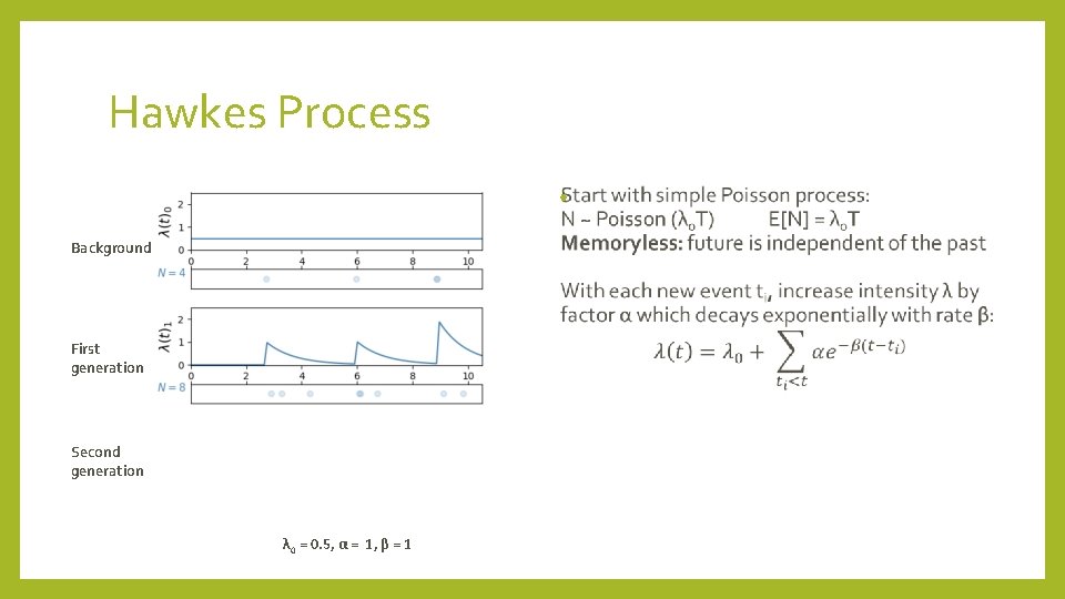
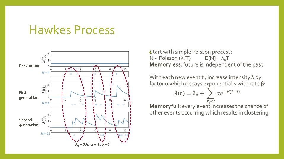
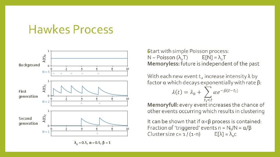
Hawkes Process Start with simple Poisson process: N ~ Poisson (λ 0 T) E[N] = λ 0 T Memoryless: future is independent of the past Background λ 0 = 0. 5

Hawkes Process • Background First generation Second generation λ 0 = 0. 5, α = 1, β = 1

Hawkes Process • Background First generation Second generation λ 0 = 0. 5, α = 1, β = 1

Hawkes Process • Background First generation Second generation λ 0 = 0. 5, α = 0. 5, β = 1

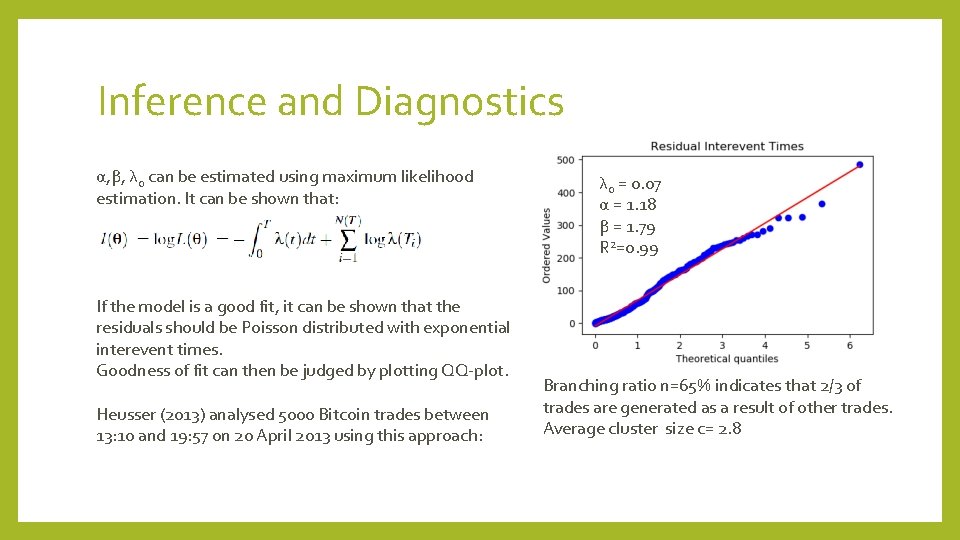
Inference and Diagnostics α, β, λ 0 can be estimated using maximum likelihood estimation. It can be shown that: If the model is a good fit, it can be shown that the residuals should be Poisson distributed with exponential interevent times. Goodness of fit can then be judged by plotting QQ-plot. Heusser (2013) analysed 5000 Bitcoin trades between 13: 10 and 19: 57 on 20 April 2013 using this approach: λ 0 = 0. 07 α = 1. 18 β = 1. 79 R 2=0. 99 Branching ratio n=65% indicates that 2/3 of trades are generated as a result of other trades. Average cluster size c= 2. 8

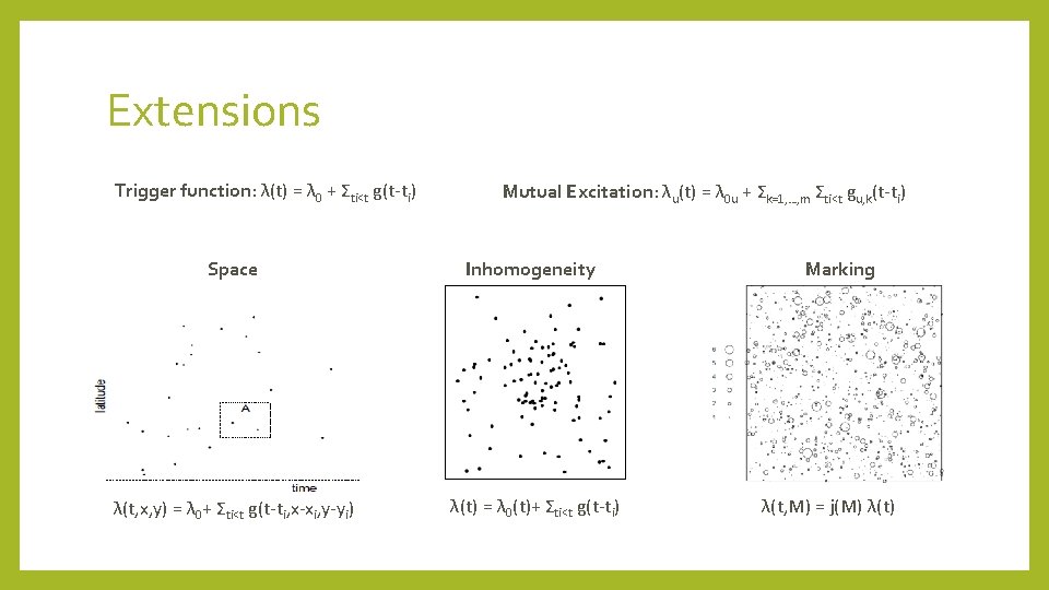
Extensions Trigger function: λ(t) = λ 0 + Σti<t g(t-ti) Mutual Excitation: λu(t) = λ 0 u + Σk=1, …, m Σti<t gu, k(t-ti) Space Inhomogeneity λ(t, x, y) = λ 0+ Σti<t g(t-ti, x-xi, y-yi) λ(t) = λ 0(t)+ Σti<t g(t-ti) Marking λ(t, M) = j(M) λ(t)

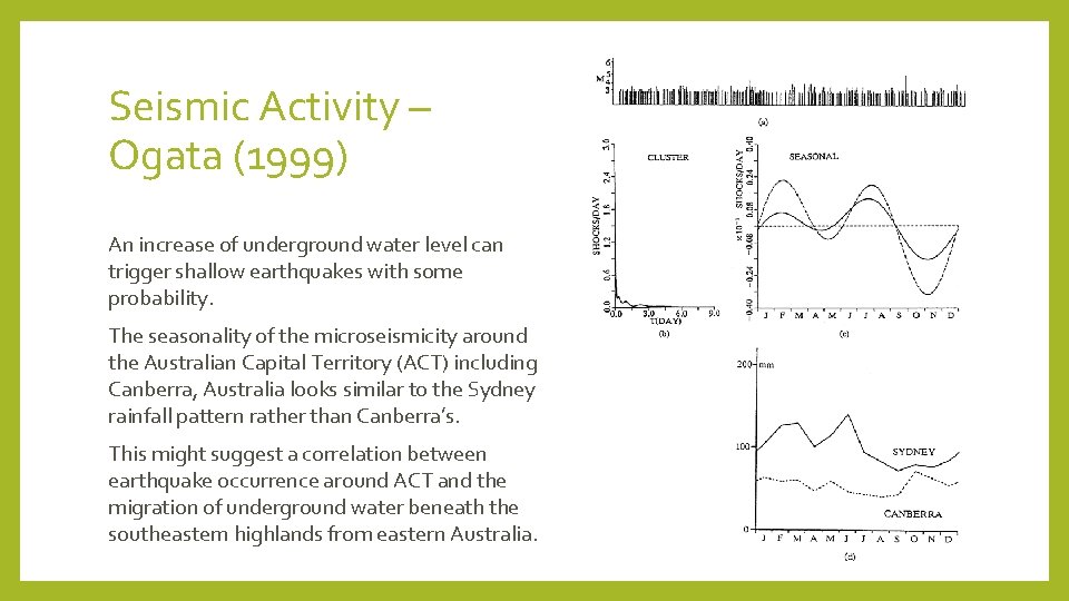
Seismic Activity – Ogata (1999) An increase of underground water level can trigger shallow earthquakes with some probability. The seasonality of the microseismicity around the Australian Capital Territory (ACT) including Canberra, Australia looks similar to the Sydney rainfall pattern rather than Canberra’s. This might suggest a correlation between earthquake occurrence around ACT and the migration of underground water beneath the southeastern highlands from eastern Australia.

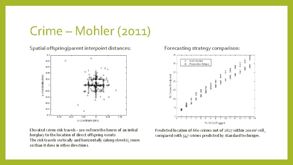
Crime – Mohler (2011) Spatial offspring/parent interpoint distances: Elevated crime risk travels ~100 m from the house of an initial burglary to the location of direct offspring events The risk travels vertically and horizontally (along streets), more so than it does in other directions. Forecasting strategy comparison: Predicted location of 660 crimes out of 2627 within 200 m 2 cell , compared with 547 crimes predicted by standard technique.

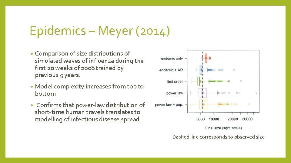
Epidemics – Meyer (2014) • Comparison of size distributions of simulated waves of influenza during the first 20 weeks of 2008 trained by previous 5 years. • Model complexity increases from top to bottom • Confirms that power-law distribution of short-time human travels translates to modelling of infectious disease spread Dashed line corresponds to observed size

Caution • Hawkes model applies only to clustered, self-exciting processes where there is an underlying generative process. • For example an infectious disease with no known carriers and where all infections can be traced back to patient ‘ 0’ cannot be modelled using the Hawkes model • MLE for estimating parameters can be computationally intensive and scale with n 2 • Many algorithms have been derived to counteract this effect • Diagnostics tools should be included in any application of the Hawkes model

References • Code for simulating and visualising Hawkes process: https: //stmorse. github. io/journal/Hawkes-python. html • Heusser (2013): http: //jheusser. github. io/2013/09/08/hawkes. html • Ogata, Y. Pure appl. geophys. (1999) 155: 471 https: //doi. org/10. 1007/s 000240050275 • G. O. Mohler et al (2011) , J. Am. Stat. Assoc. , 106: 493, 100 -108 10. 1198/jasa. 2011. ap 09546 • Meyer, Sebastian; Held, Leonhard, Ann. Appl. Stat. 8 (2014), no. 3, 1612 --1639 https: //projecteuclid. org/euclid. aoas/1414091227