Operations Research Operations Research w Operations Research OR
- Slides: 14

Operations Research

Operations Research w Operations Research (OR) aims to having the optimization solution for some administrative problems, such as transportation, decision-making, inventory Copyright 2006 John Wiley & Sons, Inc. Supplement 13 -2

Operations Research Models w Linear Programming w Markov Chains w Network Optimization w Decision Analysis w Transportation w Inventory Copyright 2006 John Wiley & Sons, Inc. Supplement 13 -3

Linear Programming (LP) A model consisting of linear relationships representing a firm’s objective and resource constraints LP is a mathematical modeling technique used to determine a level of operational activity in order to achieve an objective, subject to restrictions called constraints Copyright 2006 John Wiley & Sons, Inc. Supplement 13 -4

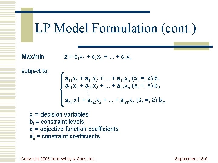
LP Model Formulation (cont. ) Max/min z = c 1 x 1 + c 2 x 2 +. . . + cnxn subject to: a 11 x 1 + a 12 x 2 +. . . + a 1 nxn (≤, =, ≥) b 1 a 21 x 1 + a 22 x 2 +. . . + a 2 nxn (≤, =, ≥) b 2 : am 1 x 1 + am 2 x 2 +. . . + amnxn (≤, =, ≥) bm xj = decision variables bi = constraint levels cj = objective function coefficients aij = constraint coefficients Copyright 2006 John Wiley & Sons, Inc. Supplement 13 -5

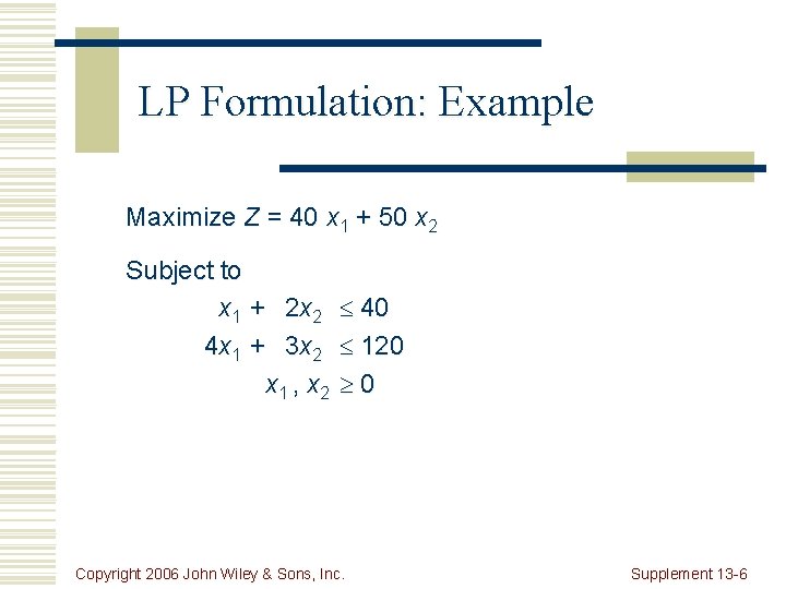
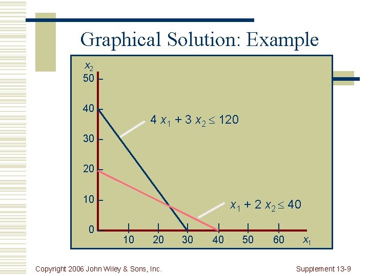
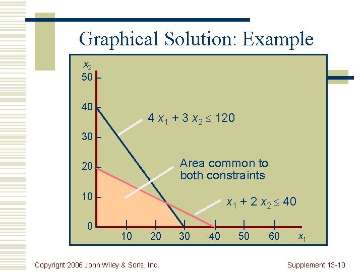
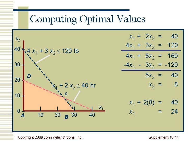
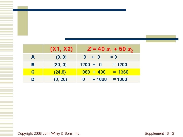
LP Formulation: Example Maximize Z = 40 x 1 + 50 x 2 Subject to x 1 + 2 x 2 4 x 1 + 3 x 2 x 1 , x 2 40 120 0 Copyright 2006 John Wiley & Sons, Inc. Supplement 13 -6

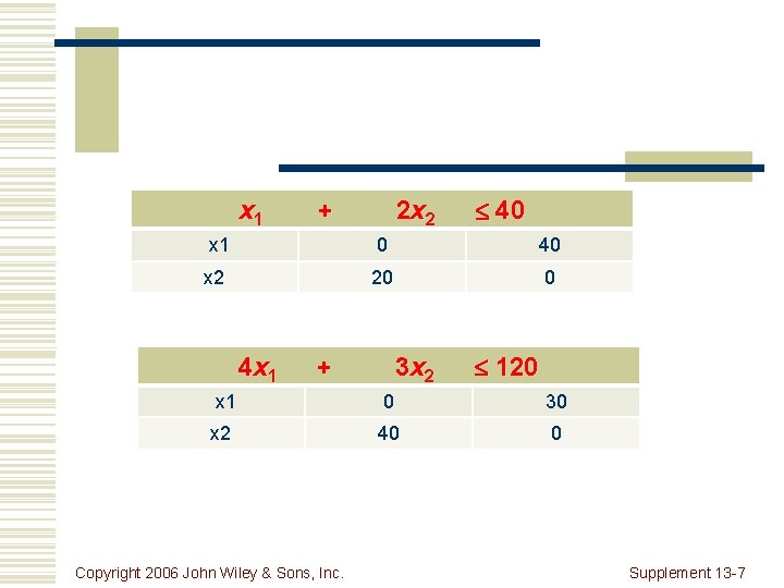
x 1 + 2 x 2 40 x 1 0 40 x 2 20 0 4 x 1 + 3 x 2 120 x 1 0 30 x 2 40 0 Copyright 2006 John Wiley & Sons, Inc. Supplement 13 -7

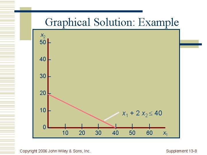
Graphical Solution: Example x 2 50 – 40 – 30 – 20 – 10 – 0– x 1 + 2 x 2 40 | 10 | 20 Copyright 2006 John Wiley & Sons, Inc. | 30 | 40 | 50 | 60 x 1 Supplement 13 -8

Graphical Solution: Example x 2 50 – 4 x 1 + 3 x 2 120 30 – 20 – 10 – 0– x 1 + 2 x 2 40 | 10 | 20 Copyright 2006 John Wiley & Sons, Inc. | 30 | 40 | 50 | 60 x 1 Supplement 13 -9

Graphical Solution: Example x 2 50 – 4 x 1 + 3 x 2 120 30 – Area common to both constraints 20 – 10 – 0– x 1 + 2 x 2 40 | 10 | 20 Copyright 2006 John Wiley & Sons, Inc. | 30 | 40 | 50 | 60 x 1 Supplement 13 -10

Computing Optimal Values x 1 + 2 x 2 = 40 4 x 1 + 3 x 2 = 120 x 2 40 – 4 x 1 + 3 x 2 120 lb 4 x 1 + 8 x 2 = 160 -4 x 1 - 3 x 2 = -120 30 – 20 – D x 1 + 2 x 2 40 hr 40 8 x 1 + 2(8) = x 1 = 40 24 c 10 – 0– A 5 x 2 = | 10 | | 20 B 30 Copyright 2006 John Wiley & Sons, Inc. | x 1 40 Supplement 13 -11

(X 1, X 2) Z = 40 x 1 + 50 x 2 A (0, 0) 0 + 0 B (30, 0) C (24, 8) 960 + 400 = 1360 D (0, 20) 0 = 1000 1200 + 0 Copyright 2006 John Wiley & Sons, Inc. + 1000 =0 = 1200 Supplement 13 -12

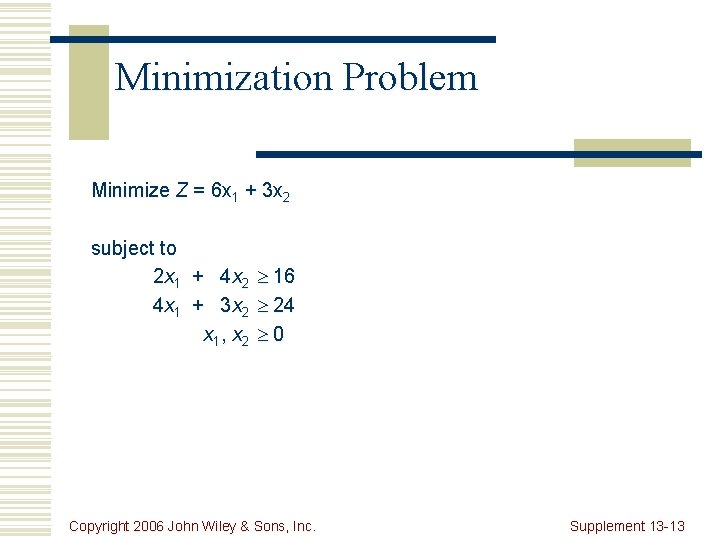
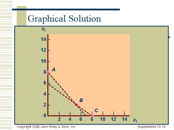
Minimization Problem Minimize Z = 6 x 1 + 3 x 2 subject to 2 x 1 + 4 x 2 4 x 1 + 3 x 2 x 1, x 2 16 24 0 Copyright 2006 John Wiley & Sons, Inc. Supplement 13 -13

Graphical Solution x 2 14 – 12 – 10 – 8–A 6– 4– B 2– 0– | 2 | 4 Copyright 2006 John Wiley & Sons, Inc. | 6 | 8 C | 10 | 12 | 14 x 1 Supplement 13 -14