Network Monitoring for Internet Traffic Engineering Jennifer Rexford

Network Monitoring for Internet Traffic Engineering Jennifer Rexford AT&T Labs – Research Florham Park, NJ 07932 http: //www. research. att. com/~jrex

Tracking the AT&T IP Backbone • Traffic – – Modem records for each World. Net dial connection SNMP link and loss statistics for every link Flow-level measurement on selective peering links Packet-level measurement on two edge links • Performance – Active probes of performance for each pair of cities • Network state – – Configuration file from each router Fault data from each router (alarms and polling) BGP routing tables for routers connecting to peers BGP update messages from two core routers

Outline • ISP backbone networks – Service provider backbone – Routing protocols • Network model for traffic engineering – Topology, capacity, and routing configuration – Destinations reachable via neighboring domains • Populating the model – Static snapshot (config files, forwarding tables) – Real-time view (OSPF monitor, i. BGP monitor) • Integration in traffic engineering tool

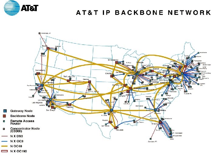
Internet Service Provider Backbone neighboring providers modem banks, business customers, web/e-mail servers Backbone routers Gateway routers Access routers

Border Gateway Protocol (BGP) • ASes exchange info about who they can reach • Update messages exchanged over a TCP connection • Local policies for path selection (which to use? ) • Local policies for route propagation (who to tell? ) • Policies configured by the AS’s network operator “I can reach 12. 34. 158. 0/23 via AS 1” “I can reach 12. 34. 158. 0/23” 2 1 3 flow of traffic 12. 34. 158. 5 AS = Autonomous System

Interior Gateway Protocol (Within an AS) • Routers flood information to learn the topology • Routers determine “next hop” to reach other routers • Path selection based on link weights (shortest path) • Link weights configured by the network operator 2 3 1 1 2 1 4 3 5 3 Path cost = 8

Traffic Engineering in an ISP Backbone • Network topology – Connectivity and capacity of routers and links • Configurable policies for resource allocation – Path selection, buffer management, and link scheduling • Traffic demands – Expected/offered load between points in the network • Performance objective – Balanced load, low latency, service level agreements … • Question: Given the topology and traffic demands, which configuration parameters should be used? This talk focuses on the topology and configuration part.

Our Approach: Measure, Model, and Control • Monitor the network to collect the various inputs • Model the network-wide path-selection process • Build tools on top of the data and the model Topology BGP updates Routing configuration Distributed routing protocols Offered traffic Flow of traffic through the network

Network Topology • Router – Loopback IP address (e. g. , 12. 123. 37. 250) – IP addresses of interfaces • Link – Network address (e. g. , 12. 125. 133. 88/30) – Capacity (e. g. , 10 Mbps, 622 Mbps) 12. 125. 133. 88/30 12. 123. 37. 250 12. 7. 108. 3 12. 125. 133. 89 12. 125. 133. 90

Core and Edge Links • Core link – OSPF weight per interface – OSPF area 1024 area 9 512 • Edge link – Set of destination prefixes {12. 34. 158. 0/23, 192. 0/24}

Populating the Model: Daily Snapshot • Router configuration files – Router name, OS version, IP address, running processes – Individual interfaces and their location in the router – Set of commands applied against the router • Processing the configuration data – Parsing the commands applied to each router – Identifying all of the outgoing interfaces at the router – Finding each pair of interfaces that forms a core link • Populates part of the model – Router, links, and link capacities – Identification of edge and core links – OSPF weights and areas for core links

Example: Router Configuration File • Language with hundreds of different commands • Cisco IOS is a de facto standard config language • Sections for interfaces, routing protocols, filters, etc. version 12. 0 hostname My. Router ! interface Loopback 0 ip address 12. 123. 37. 250 255 ! interface Serial 9/1/0/4: 0 description My. T 1 Customer bandwidth 1536 ip address 12. 125. 133. 89 255. 252 ip access-group 10 in ! interface POS 6/0 description My. Backbone. Link ip address 12. 123. 36. 73 255. 252 ip ospf cost 1024 ! router ospf network 12. 123. 36. 72 0. 0. 0. 3 area 9 network 12. 123. 37. 250 0. 0 area 9 ! access-list 10 permit 12. 125. 133. 88 0. 0. 0. 3 access-list 10 permit 135. 205. 0. 0. 255 ip route 135. 205. 0. 0 255. 0. 0 Serial 9/1/0/4: 0

Daily Snaphot: Continued • Router forwarding tables – Next-hop interface(s) for each destination prefix • Processing the forwarding tables – Identify next hops associated with edge interfaces – Ignore entries where next hop is a core interface – Extract the associated destination prefixes • Populates part of the model – Set of prefixes reachable via each edge link – Or, set of edge links associated with each prefix

Example: Forwarding Table (“show ip cef”) Prefix 4. 20. 90. 120/29 4. 20. 90. 128/29 4. 24. 7. 104/30 4. 36. 100. 0/23 6. 0. 0. 0/8 9. 2. 0. 0/16 9. 3. 4. 0/24 9. 3. 5. 0/24 9. 20. 0. 0/17 Next Hop 12. 123. 28. 134 12. 123. 28. 130 12. 123. 28. 134 192. 205. 32. 126 12. 123. 28. 134 12. 123. 28. 130 192. 205. 32. 126 12. 123. 28. 130 192. 205. 32. 178 Interface POS 7/0 POS 6/0 POS 7/0 ATM 5/0. 1 POS 7/0 POS 6/0 ATM 5/0. 1 POS 6/0 POS 0/3

Locating the Set of Egress Links for Prefix d: exit links {i, k} i Table entry: (d, i) k d Table entry: (d, k)

Populating the Model: Real-Time View • OSPF monitor – Up/down status of routers and their interfaces – OSPF weight and area for each interface • Acquiring the real-time view – Software router (Gate. D) that implements OSPF routing – Physical adjacency with an operational router – Copy of all flooded link-state advertisements Router OSPF messages Router Route monitor Work by A. Shaikh and A. Greenberg

Real-Time View (Continued) • i. BGP monitor – Destination prefixes associated with each edge link – Frequency of changes, attributes of routes, etc. • Acquiring the real-time view – Software router (Zebra) that implements BGP routing – Logical adjacency (TCP) with operational routers – “Best route” for each prefix from each vantage point Router BGP messages Route monitor BGP messages Router Work with T. Griffin and D. Caldwell

Toolkit for Traffic Engineerng • Other components of traffic engineering – Traffic measurements at destination prefix level – Path computation based on OSPF weights/areas – Network visualization to display flow of traffic – Optimization algorithm for selecting good weights Visualization Optimization Routing model Network model Traffic model

Combining With Traffic Measurements Peering point Color/size of node: proportional to traffic to this router (high to low) Color/size of link: proportional to traffic carried (high to low)

Conclusions • Summary – Network model for traffic engineering (TE) – Populating the model from existing data sets – Real-time monitoring of OSPF and BGP messages – Integration of the network model in a TE tool • Ongoing work – Extensions to support changes to BGP policies – Analysis of the real-time OSPF and BGP data – Improved support for measurement on routers • Driving goal – Accurate, timely, network-wide view of topology, routing, and traffic data

To Learn More. . . • Network overview and routing model – “Traffic engineering for IP networks” (http: //www. research. att. com/~jrex/papers/ieeenet 00. ps) • Measurement infrastructure – "Measurement and analysis of IP network usage and behavior” (http: //www. research. att. com/~jrex/papers/ieeecomm 00. ps) • Topology and configuration – “IP network configuration for intradomain traffic engineering” (http: //www. research. att. com/~jrex/papers/ieeenet 01. ps) • Traffic demands – “Deriving traffic demands for operational IP networks: Methodology and experiences” (http: //www. research. att. com/~jrex/papers/sigcomm 00. ps) • OSPF monitor – “An OSPF topology server: Design and evaluation”