NearOptimal Sensor Placements in Gaussian Processes Carlos Guestrin

Near-Optimal Sensor Placements in Gaussian Processes Carlos Guestrin Andreas Krause Carnegie Mellon University Ajit Singh

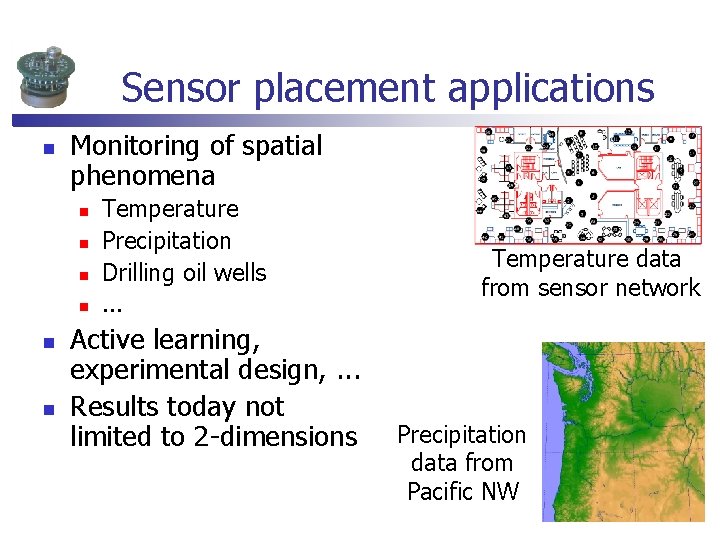
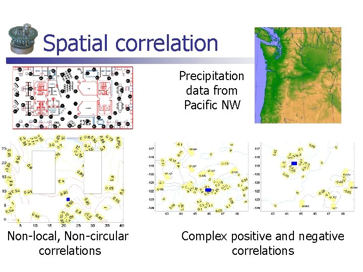
Sensor placement applications n Monitoring of spatial phenomena n n n Temperature Precipitation Drilling oil wells. . . Active learning, experimental design, . . . Results today not limited to 2 -dimensions Temperature data from sensor network Precipitation data from Pacific NW

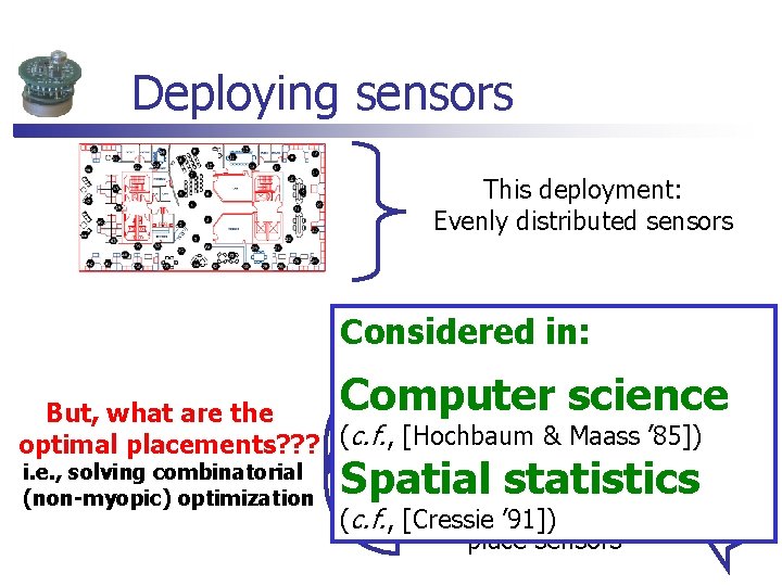
Deploying sensors This deployment: Evenly distributed sensors Chicken-and-Egg Considered in: problem: No data or assumptions about distribution But, what are the optimal placements? ? ? (c. f. , [Hochbaum & Maass ’ 85]) Computer science i. e. , solving combinatorial (non-myopic) optimization Spatial statistics Don’t know (c. f. , [Cressie ’ 91]) where to place sensors

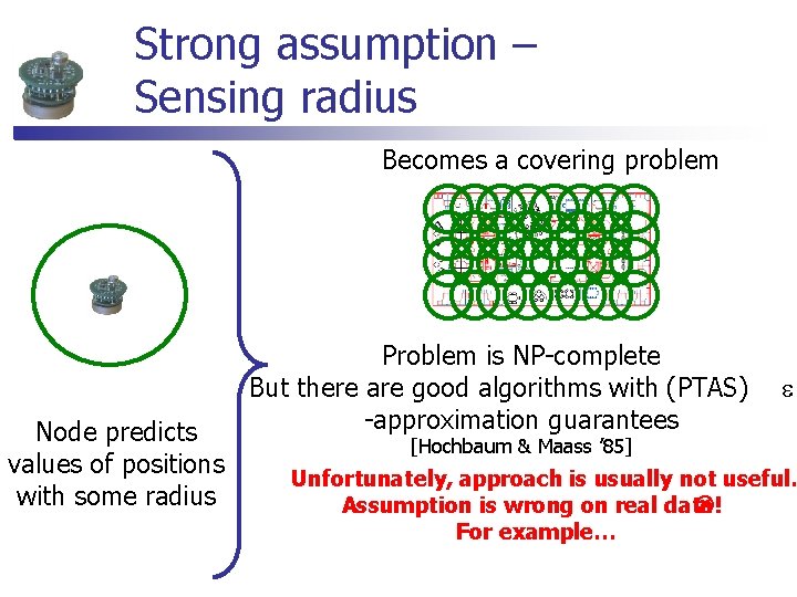
Strong assumption – Sensing radius Becomes a covering problem Node predicts values of positions with some radius Problem is NP-complete But there are good algorithms with (PTAS) -approximation guarantees [Hochbaum & Maass ’ 85] Unfortunately, approach is usually not useful… Assumption is wrong on real data! For example…

Spatial correlation Precipitation data from Pacific NW Non-local, Non-circular correlations Complex positive and negative correlations

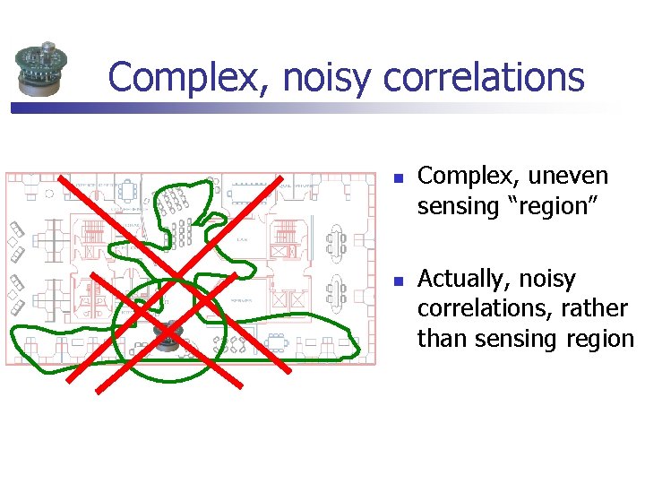
Complex, noisy correlations n n Complex, uneven sensing “region” Actually, noisy correlations, rather than sensing region

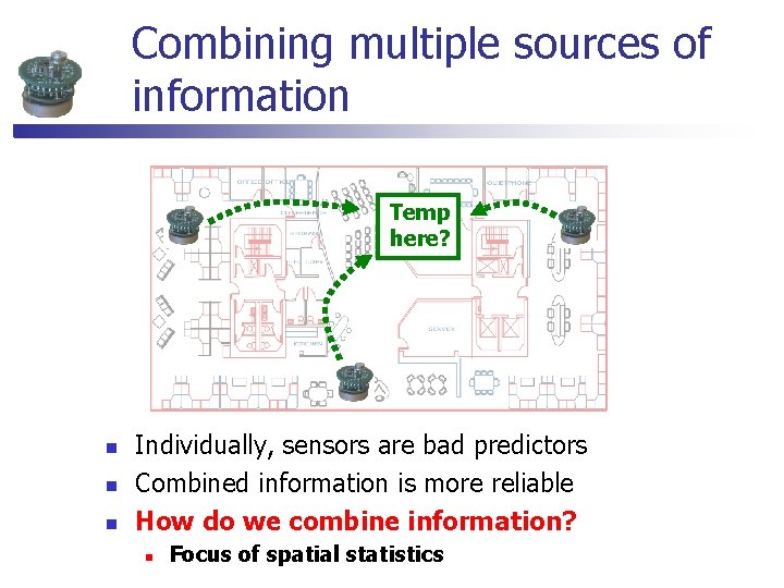
Combining multiple sources of information Temp here? n n n Individually, sensors are bad predictors Combined information is more reliable How do we combine information? n Focus of spatial statistics

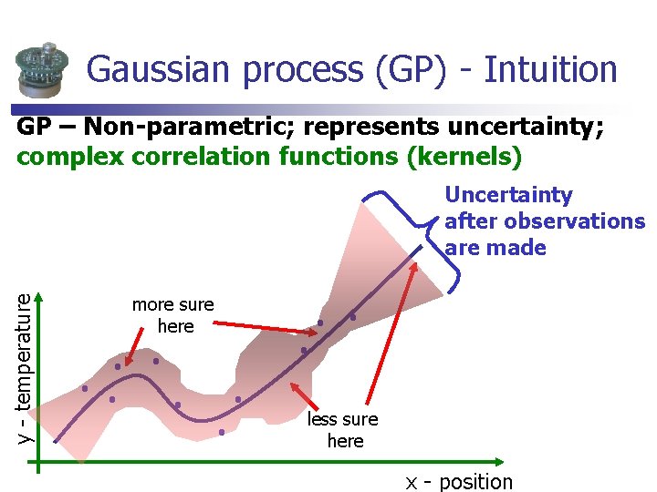
Gaussian process (GP) - Intuition GP – Non-parametric; represents uncertainty; complex correlation functions (kernels) y - temperature Uncertainty after observations are made more sure here less sure here x - position

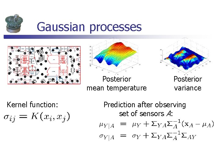
Gaussian processes Posterior mean temperature Kernel function: Posterior variance Prediction after observing set of sensors A:

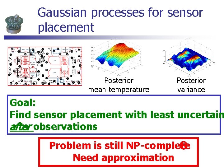
Gaussian processes for sensor placement Posterior mean temperature Posterior variance Goal: Find sensor placement with least uncertain after observations Problem is still NP-complete Need approximation

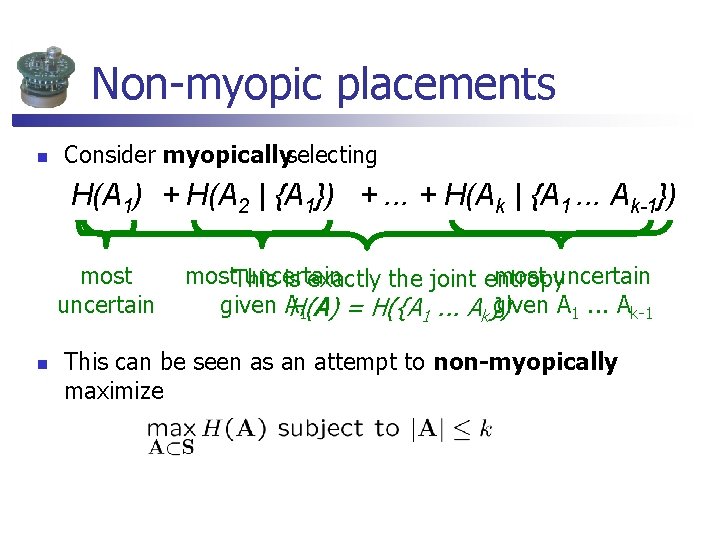
Non-myopic placements n Consider myopicallyselecting H(A 1) + H(A 2 | {A 1}) +. . . + H(Ak | {A 1. . . Ak-1}) most uncertain n most. This uncertain most uncertain is exactly the joint entropy given AH(A) given A 1. . . Ak-1 = H({A 1. . . Ak}) 1 This can be seen as an attempt to non-myopically maximize

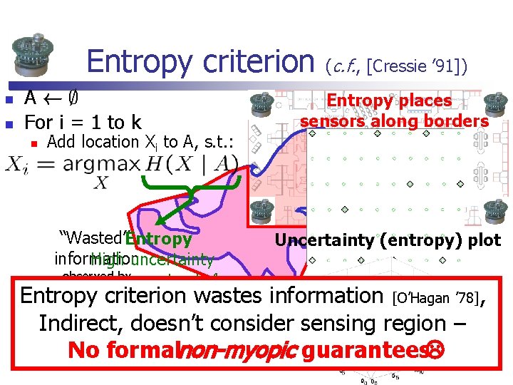
Entropy criterion n n AÃ; For i = 1 to k n (c. f. , [Cressie ’ 91]) Entropy places sensors along borders Add location Xi to A, s. t. : “Wasted”Entropy Uncertainty (entropy) plot information High uncertainty observed given by current set A – Temperature data ’ 78], [O’Hagan ’ 78] Entropy criterion wastes information [O’Hagan X is different placements: Indirect, doesn’t consider sensing Entropyregion – No formalnon-myopic guarantees

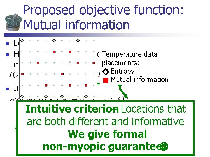
Proposed objective function: Mutual information n Locations of interest V Find locations AµV maximizing Temperature data placements: mutual information: Intuitive greedy rule: Entropy Mutual information Uncertaintyof Intuitive criterion – Locations that uninstrumented locations are both different and informative High uncertainty beforesensing. Low uncertainty after sensing We given giverestformal given A – – X is different X is informative non-myopic guarantees

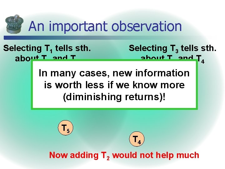
An important observation Selecting T 1 tells sth. about T 2 and T 5 Selecting T 3 tells sth. about T 2 and T 4 T 2 new information In many cases, T 1 worth less if we know more is T 3 (diminishing returns)! T 5 T 4 Now adding T 2 would not help much

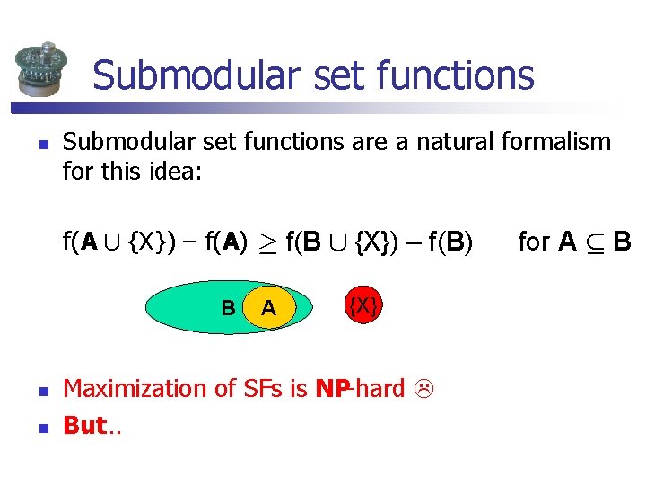
Submodular set functions n Submodular set functions are a natural formalism for this idea: f(A [ {X}) – f(A) ¸ f(B [ {X}) – f(B) B n n A {X} Maximization of SFs is NP-hard But… for A µ B

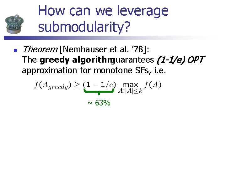
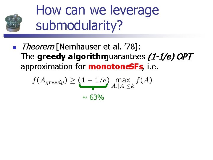
How can we leverage submodularity? n Theorem [Nemhauser et al. ’ 78]: The greedy algorithm guarantees (1 -1/e) OPT approximation for monotone SFs, i. e. ~ 63%

How can we leverage submodularity? n Theorem [Nemhauser et al. ’ 78]: The greedy algorithm guarantees (1 -1/e) OPT approximation for monotone. SFs, i. e. ~ 63%

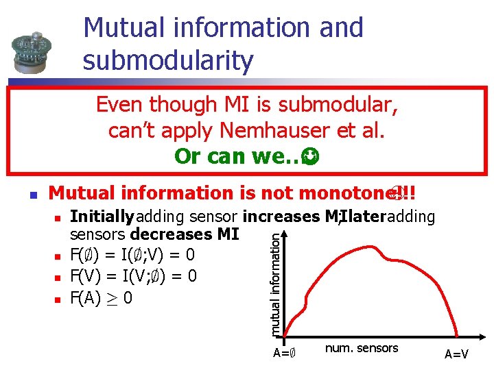
Mutual information and submodularity Mutual information submodular Even though MIis is submodular, n n n F(A) = I(A; VA) can’t apply Nemhauser et al. So, we should be able to use Nemhauser et al. Or can we… Mutual information is not monotone!!! n n Initially , adding sensor increases MI ; later adding sensors decreases MI F(; ) = I(; ; V) = 0 F(V) = I(V; ; ) = 0 F(A) ¸ 0 mutual information n A=; num. sensors A=V

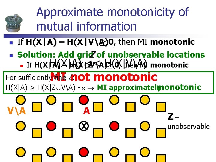
Approximate monotonicity of mutual information n If H(X|A) – H(X|VA) ¸ 0, then MI monotonic n Solution: Add grid. Z of unobservable locations n H(X|A) << H(X|VA) If H(X|A) – H(X|Z VA) ¸ 0, then MI monotonic MI not monotonic For sufficiently fine Z: H(X|A) > H(X|Z VA) - MI approximately monotonic VA A X Z– unobservable

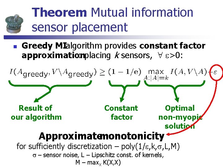
Theorem: Mutual information sensor placement n Greedy MIalgorithm provides constant factor approximation : placing k sensors, 8 >0: Result of our algorithm Constant factor Optimal non-myopic solution Approximatemonotonicity for sufficiently discretization – poly(1/ , k, , L, M) – sensor noise, L – Lipschitz const. of kernels, M – max. X K(X, X)

Different costs for different placements Theorem 1: Constant-factor approximation of optimal locations – select k sensors Theorem 2: (Cost-sensitive placements) n In practice, different locations may have different costs n n Corridor versus inside wall Have a budget. B to spend on placing sensors Constant-factor approximation – same constant (1 -1/e) n Slightly more complicated than greedy algorithm [ Sviridenko / Krause, Guestrin] n

Model learned from 54 sensors Deployment results “True” temp. prediction “True” temp. variance Mutual information has 223 new times less varianc Used initial deployment to select sensors Learned new GPthan on testentropy data using criterion just these sensors Entropy criterion Mutual information criterion Posterior mean Posterior variance

Comparing to other heuristics Greedy Our bound enables a posteriori Algorithm we analyze analysis for any heuristic n Random placements n mutual information n Better Pairwise exchange (PE) n. Assume, algorithm TUAFSPGPgives results n Start with awhich some are 10% better than the results obtained from the placement greedy algorithm n Swap locations while improving solution n. Then we immediately know, TUAFSPGP is within 70% of optimum! n

Precipitation data Better Entropy criterion Entropy Mutual information

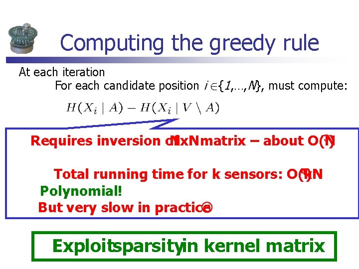
Computing the greedy rule At each iteration For each candidate position i 2{1, …, N}, must compute: 3) Requires inversion of Nx. N matrix – about O(N 4) Total running time for k sensors: O(k. N Polynomial! But very slow in practice Exploitsparsityin kernel matrix

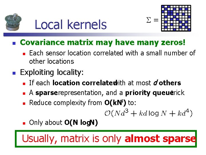
Local kernels n Covariance matrix may have many zeros! n n = Each sensor location correlated with a small number of other locations Exploiting locality: n If each location correlated with at most d others A sparserepresentation, and a priority queuetrick Reduce complexity from O(k. N 4) to: n Only about O(N log. N) n n Usually, matrix is only almost sparse

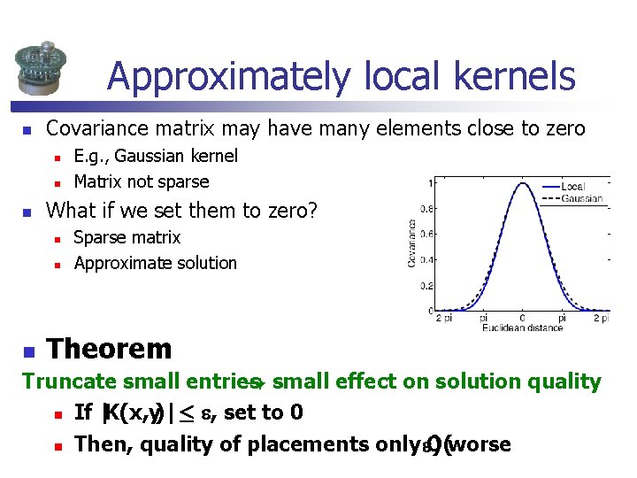
Approximately local kernels n Covariance matrix may have many elements close to zero n n n What if we set them to zero? n n n E. g. , Gaussian kernel Matrix not sparse Sparse matrix Approximate solution Theorem: Truncate small entries ! small effect on solution quality n If | K(x, y)|· , set to 0 n Then, quality of placements only ) O(worse

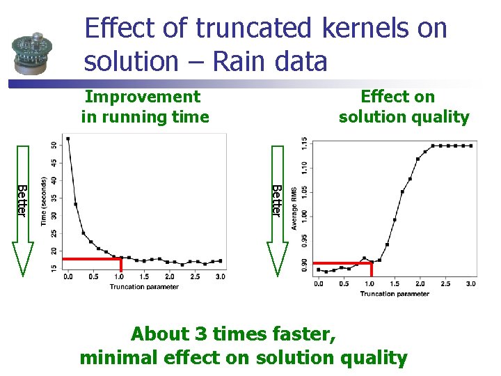
Effect of truncated kernels on solution – Rain data Improvement in running time Effect on solution quality Better About 3 times faster, minimal effect on solution quality

Summary n n n Mutual information criterion for sensor placement in general GPs Efficient algorithms with strong approximation guarantees: (1 -1/e) OPT-ε Exploiting local structureimproves efficiency Superior prediction accuracy for several real-world problems Related ideas in discrete settings presented at UAI and IJCAIthis year Effectivealgorithm for sensor placementand experimental design ; basis for active learning

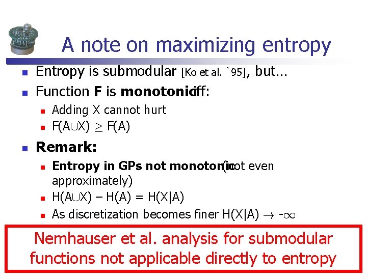
A note on maximizing entropy n n Entropy is submodular [Ko et al. `95], but… Function F is monotoniciff: n n n Adding X cannot hurt F(A[X) ¸ F(A) Remark: n n n Entropy in GPs not monotonic (not even approximately) H(A[X) – H(A) = H(X|A) As discretization becomes finer H(X|A) ! -1 Nemhauser et al. analysis for submodular functions not applicable directly to entropy

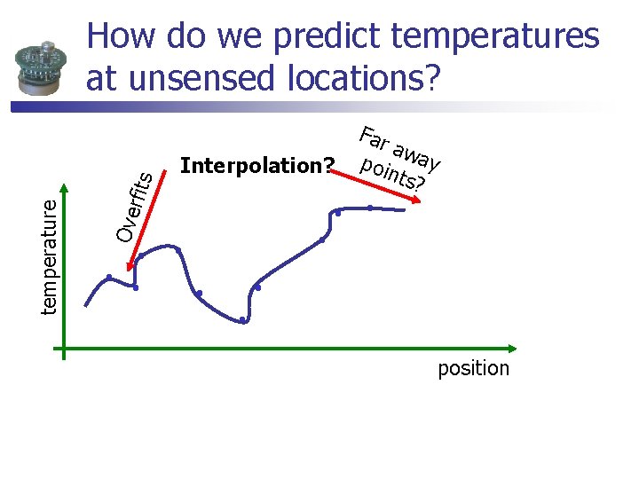
rfits Interpolation? Far awa poin y ts? Ove temperature How do we predict temperatures at unsensed locations? position

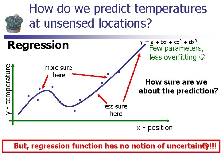
How do we predict temperatures at unsensed locations? y - temperature Regression y = a + bx + cx 2 + dx 3 Few parameters, less overfitting more sure here How sure are we about the prediction? less sure here x - position But, regression function has no notion of uncertainty!!!