Nanophotonics Atilla Ozgur Cakmak Ph D Unit 1

Nanophotonics Atilla Ozgur Cakmak, Ph. D

Unit 1 Lecture 4: Review of Quantum Physics and Introduction to Quantum Confinement-Part 2

Outline • Particle in a well • Particle in 3 -D box • Density of States

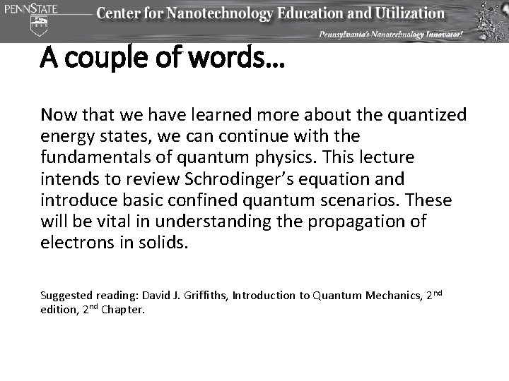
A couple of words… Now that we have learned more about the quantized energy states, we can continue with the fundamentals of quantum physics. This lecture intends to review Schrodinger’s equation and introduce basic confined quantum scenarios. These will be vital in understanding the propagation of electrons in solids. Suggested reading: David J. Griffiths, Introduction to Quantum Mechanics, 2 nd edition, 2 nd Chapter.

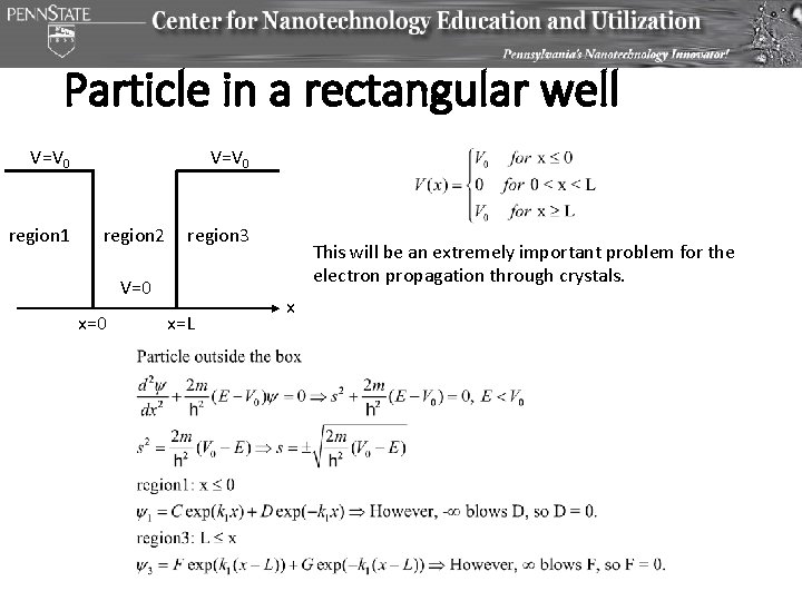
Particle in a rectangular well V=V 0 region 1 V=V 0 region 2 region 3 V=0 x=L This will be an extremely important problem for the electron propagation through crystals. x

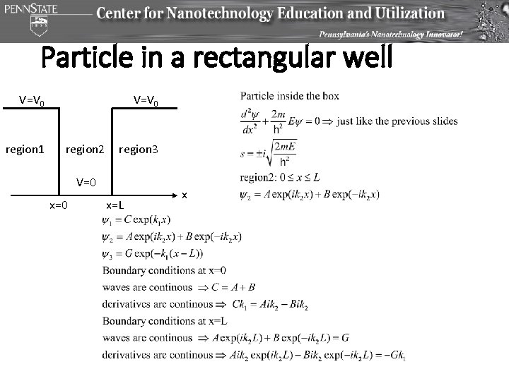
Particle in a rectangular well V=V 0 region 1 V=V 0 region 2 region 3 V=0 x=L x

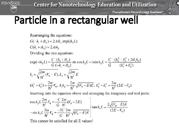
Particle in a rectangular well

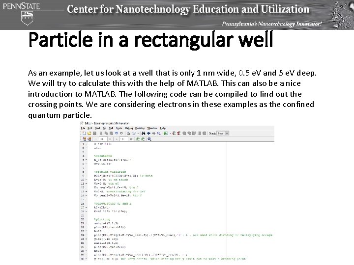
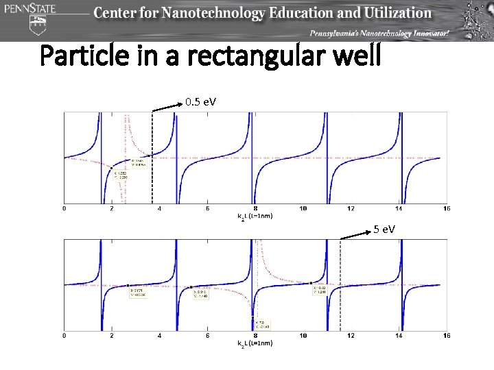
Particle in a rectangular well As an example, let us look at a well that is only 1 nm wide, 0. 5 e. V and 5 e. V deep. We will try to calculate this with the help of MATLAB. This can also be a nice introduction to MATLAB. The following code can be compiled to find out the crossing points. We are considering electrons in these examples as the confined quantum particle.

Particle in a rectangular well 0. 5 e. V

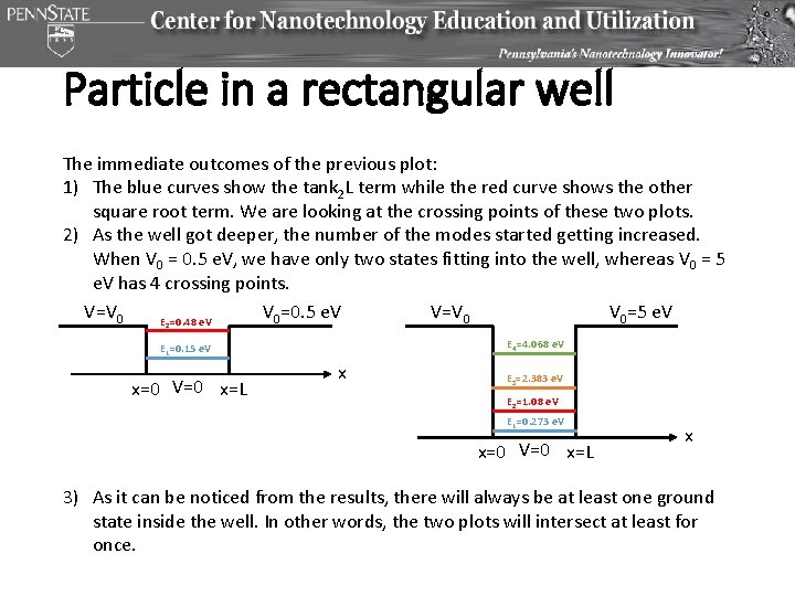
Particle in a rectangular well The immediate outcomes of the previous plot: 1) The blue curves show the tank 2 L term while the red curve shows the other square root term. We are looking at the crossing points of these two plots. 2) As the well got deeper, the number of the modes started getting increased. When V 0 = 0. 5 e. V, we have only two states fitting into the well, whereas V 0 = 5 e. V has 4 crossing points. V=V 0 V 0=0. 5 e. V V=V 0 V 0=5 e. V E =0. 48 e. V 2 E 4=4. 068 e. V E 1=0. 15 e. V x=0 V=0 x=L x E 3=2. 383 e. V E 2=1. 08 e. V E 1=0. 273 e. V x=0 V=0 x=L x 3) As it can be noticed from the results, there will always be at least one ground state inside the well. In other words, the two plots will intersect at least for once.

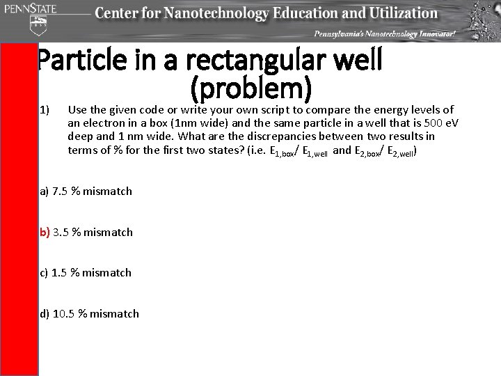
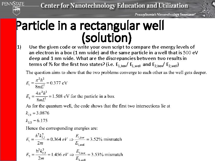
Particle in a rectangular well (problem) 1) Use the given code or write your own script to compare the energy levels of an electron in a box (1 nm wide) and the same particle in a well that is 500 e. V deep and 1 nm wide. What are the discrepancies between two results in terms of % for the first two states? (i. e. E 1, box/ E 1, well and E 2, box/ E 2, well) a) 7. 5 % mismatch b) 3. 5 % mismatch c) 1. 5 % mismatch d) 10. 5 % mismatch

Particle in a rectangular well (solution) 1) Use the given code or write your own script to compare the energy levels of an electron in a box (1 nm wide) and the same particle in a well that is 500 e. V deep and 1 nm wide. What are the discrepancies between two results in terms of % for the first two states? (i. e. E 1, box/ E 1, well and E 2, box/ E 2, well)

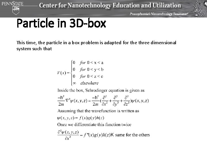
Particle in 3 D-box This time, the particle in a box problem is adapted for the three dimensional system such that

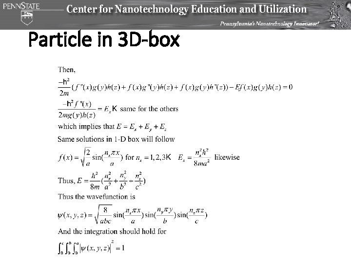
Particle in 3 D-box

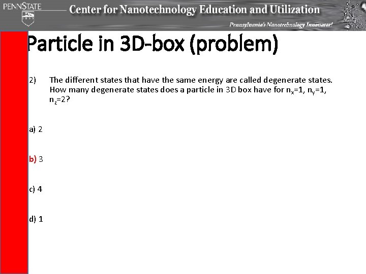
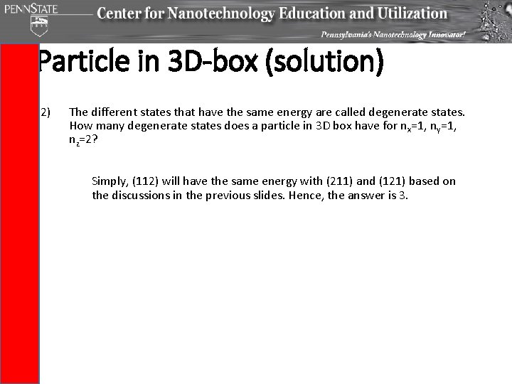
Particle in 3 D-box (problem) 2) a) 2 b) 3 c) 4 d) 1 The different states that have the same energy are called degenerate states. How many degenerate states does a particle in 3 D box have for nx=1, ny=1, nz=2?

Particle in 3 D-box (solution) 2) The different states that have the same energy are called degenerate states. How many degenerate states does a particle in 3 D box have for nx=1, ny=1, nz=2? Simply, (112) will have the same energy with (211) and (121) based on the discussions in the previous slides. Hence, the answer is 3.

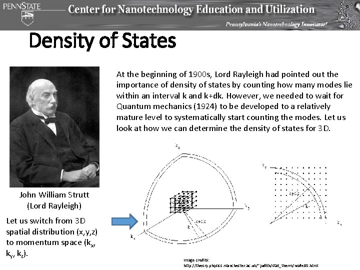
Density of States At the beginning of 1900 s, Lord Rayleigh had pointed out the importance of density of states by counting how many modes lie within an interval k and k+dk. However, we needed to wait for Quantum mechanics (1924) to be developed to a relatively mature level to systematically start counting the modes. Let us look at how we can determine the density of states for 3 D. John William Strutt (Lord Rayleigh) Let us switch from 3 D spatial distribution (x, y, z) to momentum space (kx, ky, kz). Image credits: http: //theory. physics. manchester. ac. uk/~judith/stat_therm/node 80. html

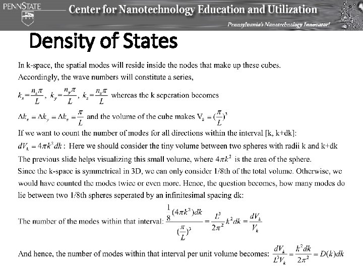
Density of States

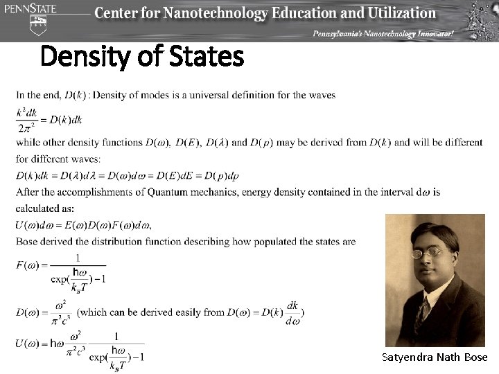
Density of States Satyendra Nath Bose

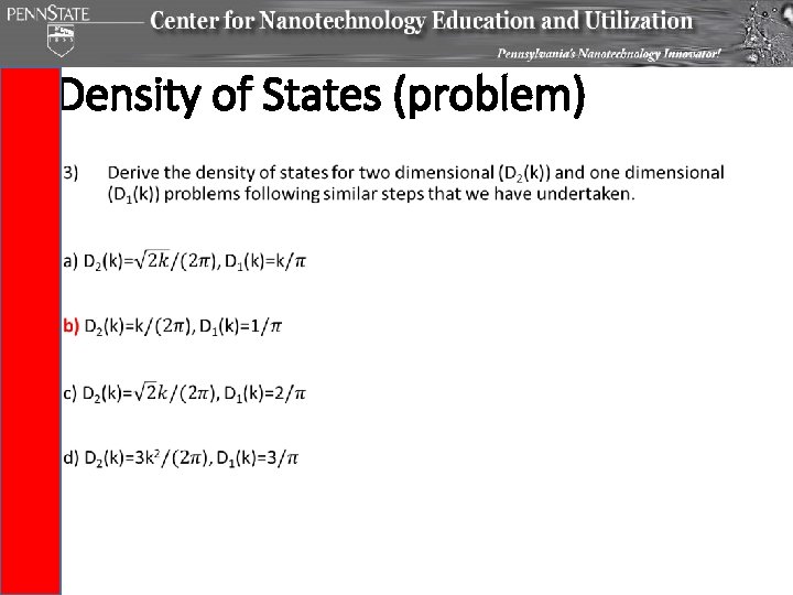
Density of States (problem) •

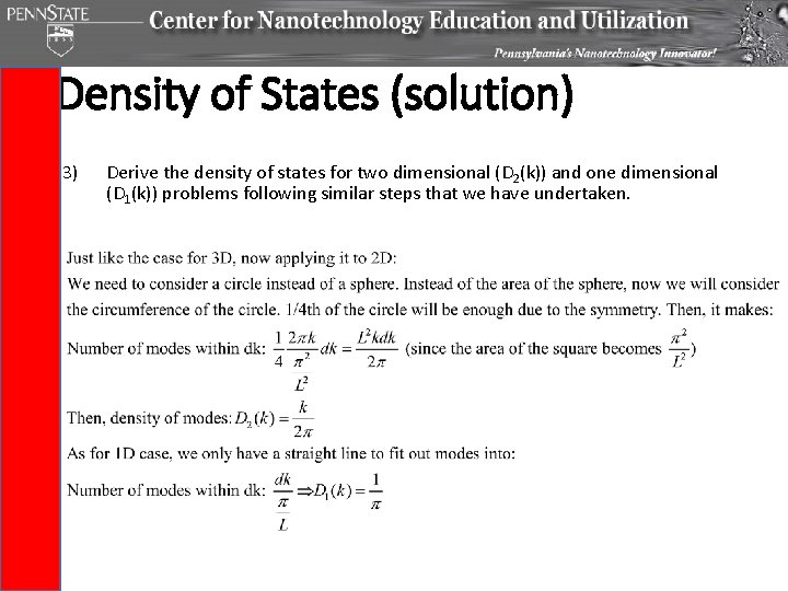
Density of States (solution) 3) Derive the density of states for two dimensional (D 2(k)) and one dimensional (D 1(k)) problems following similar steps that we have undertaken.

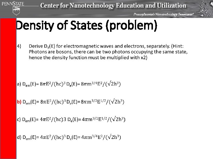
Density of States (problem) •

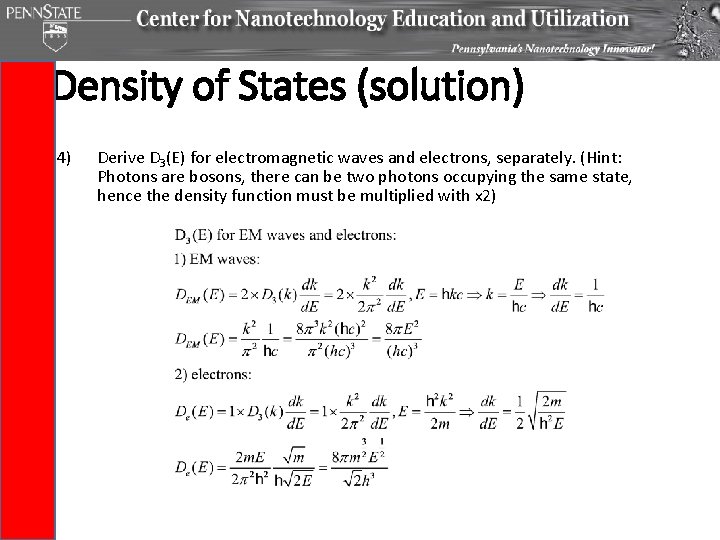
Density of States (solution) 4) Derive D 3(E) for electromagnetic waves and electrons, separately. (Hint: Photons are bosons, there can be two photons occupying the same state, hence the density function must be multiplied with x 2)