N GREGORY MANKIW PRINCIPLES OF ECONOMICS Eight Edition

N. GREGORY MANKIW PRINCIPLES OF ECONOMICS Eight Edition CHAPTE R 21 The Influence of Monetary and Fiscal Policy on Aggregate Demand Premium Power. Point Slides by: V. Andreea CHIRITESCU Eastern Illinois University © 2018 Cengage Learning®. May not be scanned, copied or duplicated, or posted to a publicly accessible website, in whole or in part, except for use as permitted in a license distributed with a certain product or service or otherwise on a password-protected website or school-approved learning management system for classroom use. 1

Look for the answers to these questions: • How does the interest-rate effect help explain the slope of the aggregate-demand curve? • How can the central bank use monetary policy to shift the AD curve? • In what two ways does fiscal policy affect aggregate demand? • What are the arguments for and against using policy to try to stabilize the economy? © 2018 Cengage Learning®. May not be scanned, copied or duplicated, or posted to a publicly accessible website, in whole or in part, except for use as permitted in a license distributed with a certain product or service or otherwise on a password-protected website or school-approved learning management system for classroom use. 2

Introduction • Earlier chapters covered: – Long-run effects of fiscal policy on interest rates, investment, economic growth – Long-run effects of monetary policy on the price level and inflation rate • This chapter focuses on – Short-run effects of fiscal and monetary policy, which work through aggregate demand © 2018 Cengage Learning®. May not be scanned, copied or duplicated, or posted to a publicly accessible website, in whole or in part, except for use as permitted in a license distributed with a certain product or service or otherwise on a password-protected website or school-approved learning management system for classroom use. 3

Aggregate Demand • Recall, the AD curve slopes downward for three reasons: – The wealth effect the most important of these effects for – The interest-rate effect the U. S. economy – The exchange-rate effect • Next: – A supply-demand model that helps explain the interest-rate effect and how monetary policy affects aggregate demand. © 2018 Cengage Learning®. May not be scanned, copied or duplicated, or posted to a publicly accessible website, in whole or in part, except for use as permitted in a license distributed with a certain product or service or otherwise on a password-protected website or school-approved learning management system for classroom use. 4

Theory of Liquidity Preference • The theory of liquidity preference – A simple theory of the interest rate (r) • r adjusts to balance supply and demand for money • Nominal interest rate, real interest rate – Assumption: expected rate of inflation is constant • Money supply: – Assumed fixed by central bank, does not depend on interest rate © 2018 Cengage Learning®. May not be scanned, copied or duplicated, or posted to a publicly accessible website, in whole or in part, except for use as permitted in a license distributed with a certain product or service or otherwise on a password-protected website or school-approved learning management system for classroom use. 5

Theory of Liquidity Preference • Money demand – Reflects how much wealth people want to hold in liquid form – Assume household wealth includes only two assets: • Money – liquid but pays no interest • Bonds – pay interest but not as liquid – A household’s “money demand” reflects its preference for liquidity © 2018 Cengage Learning®. May not be scanned, copied or duplicated, or posted to a publicly accessible website, in whole or in part, except for use as permitted in a license distributed with a certain product or service or otherwise on a password-protected website or school-approved learning management system for classroom use. 6

Theory of Liquidity Preference • Variables that influence money demand: – Y, r, and P. • Suppose real income (Y) rises: – Households want to buy more goods and services, so they need more money – To get this money, they attempt to sell some of their bonds. An increase in Y causes an increase in money demand, other things equal. © 2018 Cengage Learning®. May not be scanned, copied or duplicated, or posted to a publicly accessible website, in whole or in part, except for use as permitted in a license distributed with a certain product or service or otherwise on a password-protected website or school-approved learning management system for classroom use. 7

Active Learning 1 The determinants of money demand A. Suppose r rises, but Y and P are unchanged. What happens to money demand? B. Suppose P rises, but Y and r are unchanged. What happens to money demand? © 2018 Cengage Learning®. May not be scanned, copied or duplicated, or posted to a publicly accessible website, in whole or in part, except for use as permitted in a license distributed with a certain product or service or otherwise on a password-protected website or school-approved learning management system for classroom use. 8

Active Learning 1 Answers A. Suppose r rises, but Y and P are unchanged. What happens to money demand? – r is the opportunity cost of holding money. – An increase in r reduces money demand: households attempt to buy bonds to take advantage of the higher interest rate. – Hence, an increase in r causes a decrease in money demand, other things equal. © 2018 Cengage Learning®. May not be scanned, copied or duplicated, or posted to a publicly accessible website, in whole or in part, except for use as permitted in a license distributed with a certain product or service or otherwise on a password-protected website or school-approved learning management system for classroom use. 9

Active Learning 1 Answers B. Suppose P rises, but Y and r are unchanged. What happens to money demand? – If Y is unchanged, people will want to buy the same amount of goods and services. – Since P is higher, they will need more money to do so. – Hence, an increase in P causes an increase in money demand, other things equal. © 2018 Cengage Learning®. May not be scanned, copied or duplicated, or posted to a publicly accessible website, in whole or in part, except for use as permitted in a license distributed with a certain product or service or otherwise on a password-protected website or school-approved learning management system for classroom use. 10

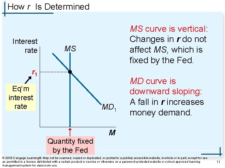
How r Is Determined Interest rate MS curve is vertical: Changes in r do not affect MS, which is fixed by the Fed. MS r 1 Eq’m interest rate MD 1 MD curve is downward sloping: A fall in r increases money demand. M Quantity fixed by the Fed © 2018 Cengage Learning®. May not be scanned, copied or duplicated, or posted to a publicly accessible website, in whole or in part, except for use as permitted in a license distributed with a certain product or service or otherwise on a password-protected website or school-approved learning management system for classroom use. 11

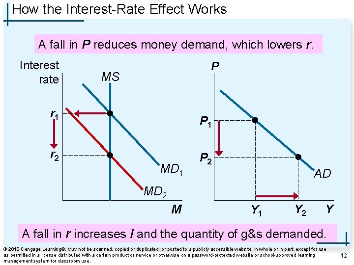
How the Interest-Rate Effect Works A fall in P reduces money demand, which lowers r. Interest rate P MS r 1 r 2 P 1 MD 1 P 2 AD MD 2 M Y 1 Y 2 Y A fall in r increases I and the quantity of g&s demanded. © 2018 Cengage Learning®. May not be scanned, copied or duplicated, or posted to a publicly accessible website, in whole or in part, except for use as permitted in a license distributed with a certain product or service or otherwise on a password-protected website or school-approved learning management system for classroom use. 12

Monetary Policy and the AD • The Fed – Use monetary policy to shift the AD curve – Policy instrument: the money supply (MS) – Targets the interest rate: the federal funds rate • Banks charge each other on short-term loans – Conducts open market operations to change MS © 2018 Cengage Learning®. May not be scanned, copied or duplicated, or posted to a publicly accessible website, in whole or in part, except for use as permitted in a license distributed with a certain product or service or otherwise on a password-protected website or school-approved learning management system for classroom use. 13

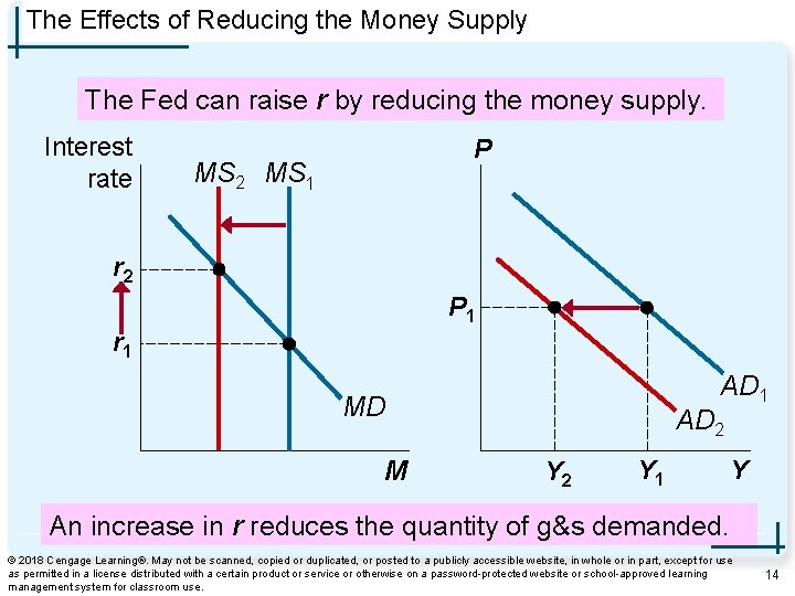
The Effects of Reducing the Money Supply The Fed can raise r by reducing the money supply. Interest rate P MS 2 MS 1 r 2 P 1 r 1 AD 1 MD M AD 2 Y 1 Y An increase in r reduces the quantity of g&s demanded. © 2018 Cengage Learning®. May not be scanned, copied or duplicated, or posted to a publicly accessible website, in whole or in part, except for use as permitted in a license distributed with a certain product or service or otherwise on a password-protected website or school-approved learning management system for classroom use. 14

Active Learning 2 Monetary policy For each of the events below, - Determine the short-run effects on output - Determine how the Fed should adjust the money supply and interest rates to stabilize output A. Congress tries to balance the budget by cutting government spending. B. A stock market boom increases household wealth. C. War breaks out in the Middle East, causing oil prices to soar. © 2018 Cengage Learning®. May not be scanned, copied or duplicated, or posted to a publicly accessible website, in whole or in part, except for use as permitted in a license distributed with a certain product or service or otherwise on a password-protected website or school-approved learning management system for classroom use. 15

Active Learning 2 Answers A. Congress tries to balance the budget by cutting government spending. – This event would reduce aggregate demand output. – To stabilize output, the Fed should increase MS and reduce r to increase aggregate demand. © 2018 Cengage Learning®. May not be scanned, copied or duplicated, or posted to a publicly accessible website, in whole or in part, except for use as permitted in a license distributed with a certain product or service or otherwise on a password-protected website or school-approved learning management system for classroom use. 16

Active Learning 2 Answers B. A stock market boom increases household wealth. – This event would increase aggregate demand, raising output above its natural rate. – To stabilize output, the Fed should reduce MS and increase r to reduce aggregate demand. © 2018 Cengage Learning®. May not be scanned, copied or duplicated, or posted to a publicly accessible website, in whole or in part, except for use as permitted in a license distributed with a certain product or service or otherwise on a password-protected website or school-approved learning management system for classroom use. 17

Active Learning 2 Answers C. War breaks out in the Middle East, causing oil prices to soar. – This event would reduce aggregate supply, causing output to fall. – To stabilize output, the Fed should increase MS and reduce r to increase aggregate demand. © 2018 Cengage Learning®. May not be scanned, copied or duplicated, or posted to a publicly accessible website, in whole or in part, except for use as permitted in a license distributed with a certain product or service or otherwise on a password-protected website or school-approved learning management system for classroom use. 18

Liquidity Traps • Liquidity trap – If interest rates have already fallen to around zero – Monetary policy may no longer be effective, since nominal interest rates cannot be reduced further • Aggregate demand, production, and employment may be "trapped" at low levels © 2018 Cengage Learning®. May not be scanned, copied or duplicated, or posted to a publicly accessible website, in whole or in part, except for use as permitted in a license distributed with a certain product or service or otherwise on a password-protected website or school-approved learning management system for classroom use. 19

Liquidity Traps • A central bank continues to have tools to expand the economy: – Forward guidance: raise inflation expectations by committing to keep interest rates low – Quantitative easing: buy a larger variety of financial instruments (mortgages, corporate debt, and longer-term government bonds) (The Fed, 2008) © 2018 Cengage Learning®. May not be scanned, copied or duplicated, or posted to a publicly accessible website, in whole or in part, except for use as permitted in a license distributed with a certain product or service or otherwise on a password-protected website or school-approved learning management system for classroom use. 20

Fiscal Policy and the AD • Fiscal policy: – Setting the level of government spending and taxation by government policymakers – Expansionary fiscal policy • An increase in G and/or decrease in T, shifts AD right – Contractionary fiscal policy • A decrease in G and/or increase in T, shifts AD left • Fiscal policy has two effects on AD. . . © 2018 Cengage Learning®. May not be scanned, copied or duplicated, or posted to a publicly accessible website, in whole or in part, except for use as permitted in a license distributed with a certain product or service or otherwise on a password-protected website or school-approved learning management system for classroom use. 21

1. The Multiplier Effect • Example: If the government buys $20 b of planes from Boeing, Boeing’s revenue increases by $20 b. – This is distributed to Boeing’s workers (as wages) and owners (as profits or stock dividends). – These people are also consumers and will spend a portion of the extra income. – This extra consumption causes further increases in aggregate demand. © 2018 Cengage Learning®. May not be scanned, copied or duplicated, or posted to a publicly accessible website, in whole or in part, except for use as permitted in a license distributed with a certain product or service or otherwise on a password-protected website or school-approved learning management system for classroom use. 22

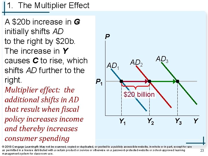
1. The Multiplier Effect A $20 b increase in G initially shifts AD P to the right by $20 b. The increase in Y AD 3 causes C to rise, which AD 2 AD 1 shifts AD further to the right. P 1 Multiplier effect: the $20 billion additional shifts in AD that result when fiscal policy increases income Y 2 Y 3 Y 1 and thereby increases consumer spending © 2018 Cengage Learning®. May not be scanned, copied or duplicated, or posted to a publicly accessible website, in whole or in part, except for use as permitted in a license distributed with a certain product or service or otherwise on a password-protected website or school-approved learning management system for classroom use. Y 23

Marginal Propensity to Consume • How big is the multiplier effect? – Depends on how much consumers respond to increases in income. • Marginal propensity to consume, MPC=ΔC/ΔY – Fraction of extra income that households consume rather than save • Example – If MPC = 0. 8 and income rises $100, C rises $80. © 2018 Cengage Learning®. May not be scanned, copied or duplicated, or posted to a publicly accessible website, in whole or in part, except for use as permitted in a license distributed with a certain product or service or otherwise on a password-protected website or school-approved learning management system for classroom use. 24

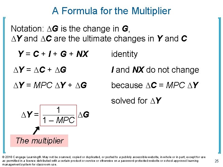
A Formula for the Multiplier Notation: ΔG is the change in G, ΔY and ΔC are the ultimate changes in Y and C Y = C + I + G + NX identity ΔY = ΔC + ΔG I and NX do not change ΔY = MPC ΔY + ΔG because ΔC = MPC ΔY 1 ΔY = ΔG 1 – MPC solved for ΔY The multiplier © 2018 Cengage Learning®. May not be scanned, copied or duplicated, or posted to a publicly accessible website, in whole or in part, except for use as permitted in a license distributed with a certain product or service or otherwise on a password-protected website or school-approved learning management system for classroom use. 25

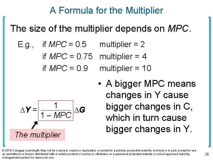
A Formula for the Multiplier The size of the multiplier depends on MPC. E. g. , if MPC = 0. 5 multiplier = 2 if MPC = 0. 75 multiplier = 4 if MPC = 0. 9 multiplier = 10 1 ΔY = ΔG 1 – MPC The multiplier • A bigger MPC means changes in Y cause bigger changes in C, which in turn cause bigger changes in Y. © 2018 Cengage Learning®. May not be scanned, copied or duplicated, or posted to a publicly accessible website, in whole or in part, except for use as permitted in a license distributed with a certain product or service or otherwise on a password-protected website or school-approved learning management system for classroom use. 26

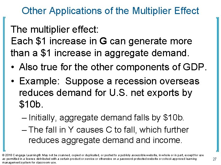
Other Applications of the Multiplier Effect The multiplier effect: Each $1 increase in G can generate more than a $1 increase in aggregate demand. • Also true for the other components of GDP. • Example: Suppose a recession overseas reduces demand for U. S. net exports by $10 b. – Initially, aggregate demand falls by $10 b. – The fall in Y causes C to fall, which further reduces aggregate demand income. © 2018 Cengage Learning®. May not be scanned, copied or duplicated, or posted to a publicly accessible website, in whole or in part, except for use as permitted in a license distributed with a certain product or service or otherwise on a password-protected website or school-approved learning management system for classroom use. 27

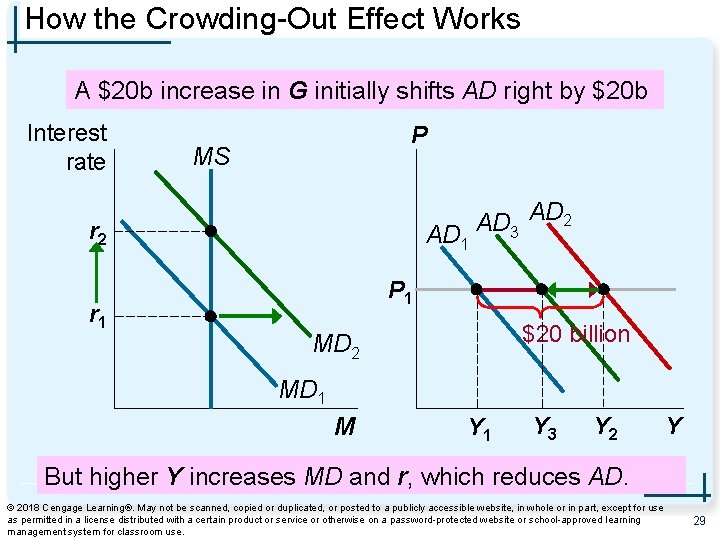
2. The Crowding-Out Effect • The crowding-out effect – Offset in aggregate demand – Results when expansionary fiscal policy raises the interest rate – Thereby reduces investment spending – Which reduces the net increase in aggregate demand. – So, the size of the AD shift may be smaller than the initial fiscal expansion. © 2018 Cengage Learning®. May not be scanned, copied or duplicated, or posted to a publicly accessible website, in whole or in part, except for use as permitted in a license distributed with a certain product or service or otherwise on a password-protected website or school-approved learning management system for classroom use. 28

How the Crowding-Out Effect Works A $20 b increase in G initially shifts AD right by $20 b Interest rate P MS AD 2 AD 3 AD 1 r 2 r 1 P 1 $20 billion MD 2 MD 1 M Y 1 Y 3 Y 2 Y But higher Y increases MD and r, which reduces AD. © 2018 Cengage Learning®. May not be scanned, copied or duplicated, or posted to a publicly accessible website, in whole or in part, except for use as permitted in a license distributed with a certain product or service or otherwise on a password-protected website or school-approved learning management system for classroom use. 29

Changes in Taxes • A tax cut – Increases households’ take-home pay – Households respond by spending a portion of this extra income, shifting AD to the right – The size of the shift is affected by the multiplier and crowding-out effects • Another factor: households perception – Permanent tax cut – large impact on AD – Temporary tax cut – small impact on AD © 2018 Cengage Learning®. May not be scanned, copied or duplicated, or posted to a publicly accessible website, in whole or in part, except for use as permitted in a license distributed with a certain product or service or otherwise on a password-protected website or school-approved learning management system for classroom use. 30

Active Learning 3 Fiscal policy effects The economy is in recession. Shifting the AD curve rightward by $200 b would end the recession. A. If MPC =. 8 and there is no crowding out, how much should Congress increase G to end the recession? B. If there is crowding out, will Congress need to increase G more or less than this amount? © 2018 Cengage Learning®. May not be scanned, copied or duplicated, or posted to a publicly accessible website, in whole or in part, except for use as permitted in a license distributed with a certain product or service or otherwise on a password-protected website or school-approved learning management system for classroom use. 31

Active Learning 3 Answers The economy is in recession. Shifting the AD curve rightward by $200 b would end the recession. A. If MPC =. 8 and there is no crowding out, how much should Congress increase G to end the recession? – Multiplier = 1/(1 –. 8) = 5 – Increase G by $40 b to shift aggregate demand by 5 x $40 b = $200 b. © 2018 Cengage Learning®. May not be scanned, copied or duplicated, or posted to a publicly accessible website, in whole or in part, except for use as permitted in a license distributed with a certain product or service or otherwise on a password-protected website or school-approved learning management system for classroom use. 32

Active Learning 3 Answers The economy is in recession. Shifting the AD curve rightward by $200 b would end the recession. B. If there is crowding out, will Congress need to increase G more or less than this amount? – Crowding out reduces the impact of G on AD. – To offset this, Congress should increase G by a larger amount. © 2018 Cengage Learning®. May not be scanned, copied or duplicated, or posted to a publicly accessible website, in whole or in part, except for use as permitted in a license distributed with a certain product or service or otherwise on a password-protected website or school-approved learning management system for classroom use. 33

Fiscal Policy and Aggregate Supply Fiscal policy might affect aggregate supply People respond to incentives • A cut in the tax rate – Gives workers incentive to work more, so it might increase the quantity of goods and services supplied and shift AS to the right. – People who believe this effect is large are called “Supply-siders” © 2018 Cengage Learning®. May not be scanned, copied or duplicated, or posted to a publicly accessible website, in whole or in part, except for use as permitted in a license distributed with a certain product or service or otherwise on a password-protected website or school-approved learning management system for classroom use. 34

Fiscal Policy and Aggregate Supply G might affect aggregate supply. • Example: government increases spending on roads. – Better roads may increase business productivity, which increases the quantity of goods and services supplied, shifts AS to the right – This effect is probably more relevant in the long run: it takes time to build the new roads and put them into use © 2018 Cengage Learning®. May not be scanned, copied or duplicated, or posted to a publicly accessible website, in whole or in part, except for use as permitted in a license distributed with a certain product or service or otherwise on a password-protected website or school-approved learning management system for classroom use. 35

The Case for Active Stabilization Policy • Keynes: “Animal spirits” cause waves of pessimism and optimism among households and firms, leading to shifts in aggregate demand fluctuations in output and employment. • Also, other factors cause fluctuations, – Booms and recessions abroad – Stock market booms and crashes • If policymakers do nothing – These fluctuations are destabilizing to businesses, workers, consumers. © 2018 Cengage Learning®. May not be scanned, copied or duplicated, or posted to a publicly accessible website, in whole or in part, except for use as permitted in a license distributed with a certain product or service or otherwise on a password-protected website or school-approved learning management system for classroom use. 36

The Case for Active Stabilization Policy • Proponents of active stabilization policy – Government should use policy to reduce these fluctuations: • When GDP falls below its natural rate, use expansionary monetary or fiscal policy to prevent or reduce a recession. • When GDP rises above its natural rate, use contractionary policy to prevent or reduce an inflationary boom © 2018 Cengage Learning®. May not be scanned, copied or duplicated, or posted to a publicly accessible website, in whole or in part, except for use as permitted in a license distributed with a certain product or service or otherwise on a password-protected website or school-approved learning management system for classroom use. 37

Keynesians in the White House • 1961, John F Kennedy – Pushed for a tax cut to stimulate aggregate demand – Several of his economic advisors were followers of Keynes • 2009, President Barak Obama – Economy in recession – Policy: stimulus bill - the American Recovery and Reinvestment Act (ARRA), • Substantial increase in government spending © 2018 Cengage Learning®. May not be scanned, copied or duplicated, or posted to a publicly accessible website, in whole or in part, except for use as permitted in a license distributed with a certain product or service or otherwise on a password-protected website or school-approved learning management system for classroom use. 38

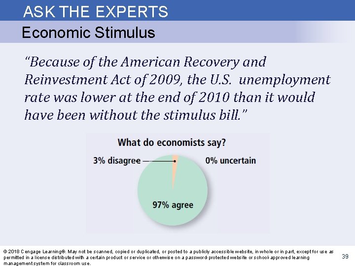
ASK THE EXPERTS Economic Stimulus “Because of the American Recovery and Reinvestment Act of 2009, the U. S. unemployment rate was lower at the end of 2010 than it would have been without the stimulus bill. ” © 2018 Cengage Learning®. May not be scanned, copied or duplicated, or posted to a publicly accessible website, in whole or in part, except for use as permitted in a license distributed with a certain product or service or otherwise on a password-protected website or school-approved learning management system for classroom use. 39

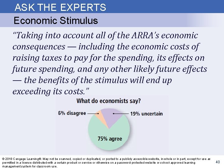
ASK THE EXPERTS Economic Stimulus “Taking into account all of the ARRA’s economic consequences — including the economic costs of raising taxes to pay for the spending, its effects on future spending, and any other likely future effects — the benefits of the stimulus will end up exceeding its costs. ” © 2018 Cengage Learning®. May not be scanned, copied or duplicated, or posted to a publicly accessible website, in whole or in part, except for use as permitted in a license distributed with a certain product or service or otherwise on a password-protected website or school-approved learning management system for classroom use. 40

The Case Against Active Stabilization Policy • Monetary policy affects economy with a long lag: – Firms make investment plans in advance, so I takes time to respond to changes in r – Most economists believe it takes at least 6 months for mon policy to affect output and employment • Fiscal policy also works with a long lag: – Changes in G and T require acts of Congress. – Legislative process can take months or years © 2018 Cengage Learning®. May not be scanned, copied or duplicated, or posted to a publicly accessible website, in whole or in part, except for use as permitted in a license distributed with a certain product or service or otherwise on a password-protected website or school-approved learning management system for classroom use. 41

The Case Against Active Stabilization Policy • Due to these long lags – Critics of active policy argue that such policies may destabilize the economy rather than help it: • By the time the policies affect aggregate demand, the economy’s condition may have changed. • Contend that policymakers should focus on long-run goals like economic growth and low inflation. © 2018 Cengage Learning®. May not be scanned, copied or duplicated, or posted to a publicly accessible website, in whole or in part, except for use as permitted in a license distributed with a certain product or service or otherwise on a password-protected website or school-approved learning management system for classroom use. 42

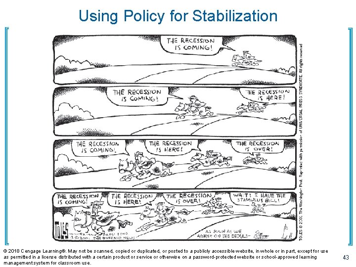
Using Policy for Stabilization © 2018 Cengage Learning®. May not be scanned, copied or duplicated, or posted to a publicly accessible website, in whole or in part, except for use as permitted in a license distributed with a certain product or service or otherwise on a password-protected website or school-approved learning management system for classroom use. 43

Automatic Stabilizers • Automatic stabilizers: – Changes in fiscal policy that stimulate aggregate demand when economy goes into recession – Without policymakers having to take any deliberate action © 2018 Cengage Learning®. May not be scanned, copied or duplicated, or posted to a publicly accessible website, in whole or in part, except for use as permitted in a license distributed with a certain product or service or otherwise on a password-protected website or school-approved learning management system for classroom use. 44

Automatic Stabilizers: Examples • The tax system – In recession, taxes fall automatically, which stimulates aggregate demand • Government spending – In recession, more people apply for public assistance (welfare, unemployment insurance) • Government spending on these programs automatically rises, which stimulates aggregate demand © 2018 Cengage Learning®. May not be scanned, copied or duplicated, or posted to a publicly accessible website, in whole or in part, except for use as permitted in a license distributed with a certain product or service or otherwise on a password-protected website or school-approved learning management system for classroom use. 45

Conclusion • When Congress cuts taxes – Should consider the short-run effects on aggregate demand employment – And the long-run effects on saving and growth • When the Fed reduces the rate of money growth – Must take into account not only the long-run effects on inflation – But the short-run effects on output and employment © 2018 Cengage Learning®. May not be scanned, copied or duplicated, or posted to a publicly accessible website, in whole or in part, except for use as permitted in a license distributed with a certain product or service or otherwise on a password-protected website or school-approved learning management system for classroom use. 46

Summary • Theory of liquidity preference: the interest rate • adjusts to balance the demand for money with the supply of money. The interest-rate effect helps explain why the aggregate-demand curve slopes downward: • An increase in the price level raises money demand, which raises the interest rate, which reduces investment, which reduces the aggregate quantity of goods & services demanded. © 2018 Cengage Learning®. May not be scanned, copied or duplicated, or posted to a publicly accessible website, in whole or in part, except for use as permitted in a license distributed with a certain product or service or otherwise on a password-protected website or school-approved learning management system for classroom use. 47

Summary • An increase in the money supply causes the • interest rate to fall, which stimulates investment and shifts the aggregate demand curve rightward. Expansionary fiscal policy—a spending increase or tax cut—shifts aggregate demand to the right. Contractionary fiscal policy shifts aggregate demand to the left. © 2018 Cengage Learning®. May not be scanned, copied or duplicated, or posted to a publicly accessible website, in whole or in part, except for use as permitted in a license distributed with a certain product or service or otherwise on a password-protected website or school-approved learning management system for classroom use. 48

Summary • When the government alters spending or taxes, the resulting shift in aggregate demand can be larger or smaller than the fiscal change: • The multiplier effect tends to amplify the effects • of fiscal policy on aggregate demand. The crowding-out effect tends to dampen the effects of fiscal policy on aggregate demand. © 2018 Cengage Learning®. May not be scanned, copied or duplicated, or posted to a publicly accessible website, in whole or in part, except for use as permitted in a license distributed with a certain product or service or otherwise on a password-protected website or school-approved learning management system for classroom use. 49

Summary • Economists disagree about how actively • • policymakers should try to stabilize the economy. Some argue that the government should use fiscal and monetary policy to combat destabilizing fluctuations in output and employment. Others argue that policy will end up destabilizing the economy because policies work with long lags. © 2018 Cengage Learning®. May not be scanned, copied or duplicated, or posted to a publicly accessible website, in whole or in part, except for use as permitted in a license distributed with a certain product or service or otherwise on a password-protected website or school-approved learning management system for classroom use. 50