MSc Methods XX YY Dr Mathias Mat Disney

MSc Methods XX: YY Dr. Mathias (Mat) Disney UCL Geography Office: 113, Pearson Building Tel: 7670 0592 Email: mdisney@ucl. geog. ac. uk www. geog. ucl. ac. uk/~mdisney

Lecture outline • Two parameter estimation – Some stuff • Uncertainty & linear approximations – parameter estimation, uncertainty – Practical – basic Bayesian estimation • Linear Models – parameter estimation, uncertainty – Practical – basic Bayesian estimation

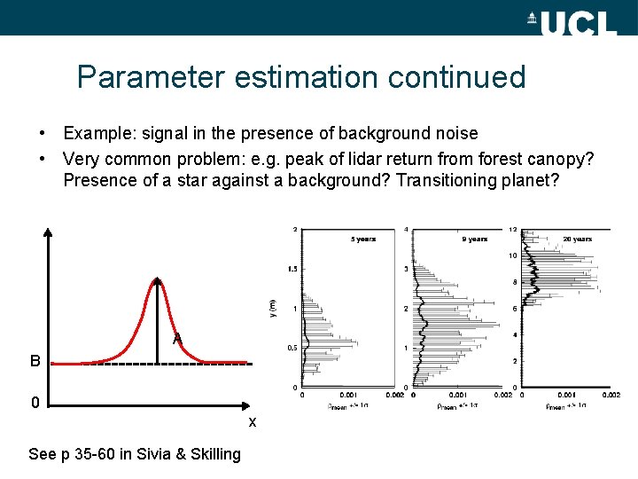
Parameter estimation continued • Example: signal in the presence of background noise • Very common problem: e. g. peak of lidar return from forest canopy? Presence of a star against a background? Transitioning planet? A B 0 x See p 35 -60 in Sivia & Skilling

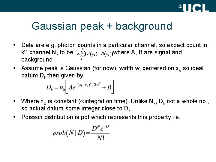
Gaussian peak + background • Data are e. g. photon counts in a particular channel, so expect count in kth channel Nk to be where A, B are signal and background • Assume peak is Gaussian (for now), width w, centered on xo so ideal datum Dk then given by • Where n 0 is constant ( integration time). Unlike Nk, Dk not a whole no. , so actual datum some integer close to Dk • Poisson distribution is pdf which represents this property i. e.

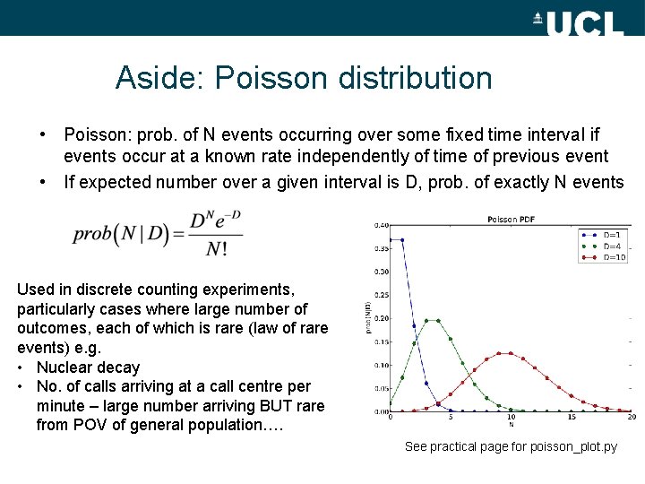
Aside: Poisson distribution • Poisson: prob. of N events occurring over some fixed time interval if events occur at a known rate independently of time of previous event • If expected number over a given interval is D, prob. of exactly N events Used in discrete counting experiments, particularly cases where large number of outcomes, each of which is rare (law of rare events) e. g. • Nuclear decay • No. of calls arriving at a call centre per minute – large number arriving BUT rare from POV of general population…. See practical page for poisson_plot. py

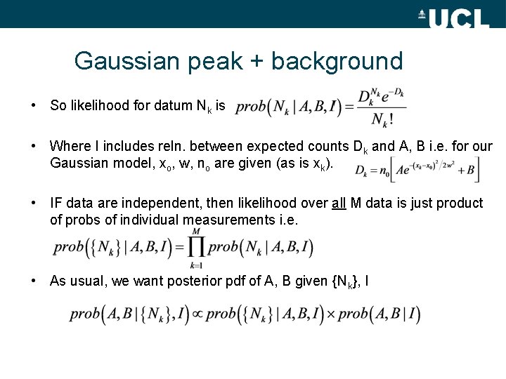
Gaussian peak + background • So likelihood for datum Nk is • Where I includes reln. between expected counts Dk and A, B i. e. for our Gaussian model, xo, w, no are given (as is xk). • IF data are independent, then likelihood over all M data is just product of probs of individual measurements i. e. • As usual, we want posterior pdf of A, B given {Nk}, I

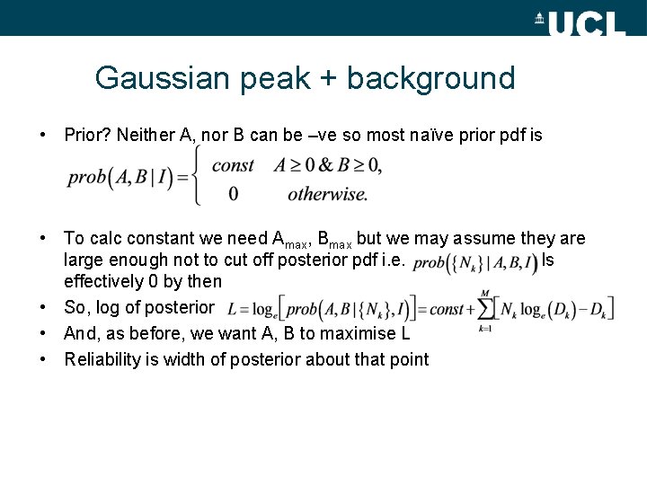
Gaussian peak + background • Prior? Neither A, nor B can be –ve so most naïve prior pdf is • To calc constant we need Amax, Bmax but we may assume they are large enough not to cut off posterior pdf i. e. Is effectively 0 by then • So, log of posterior • And, as before, we want A, B to maximise L • Reliability is width of posterior about that point

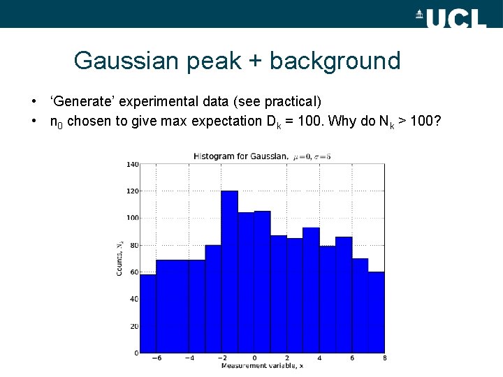
Gaussian peak + background • ‘Generate’ experimental data (see practical) • n 0 chosen to give max expectation Dk = 100. Why do Nk > 100?

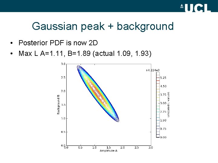
Gaussian peak + background • Posterior PDF is now 2 D • Max L A=1. 11, B=1. 89 (actual 1. 09, 1. 93)

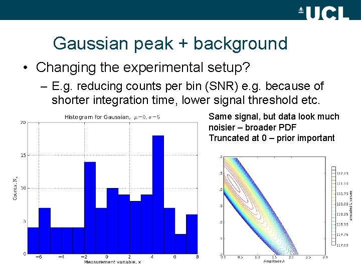
Gaussian peak + background • Changing the experimental setup? – E. g. reducing counts per bin (SNR) e. g. because of shorter integration time, lower signal threshold etc. Same signal, but data look much noisier – broader PDF Truncated at 0 – prior important

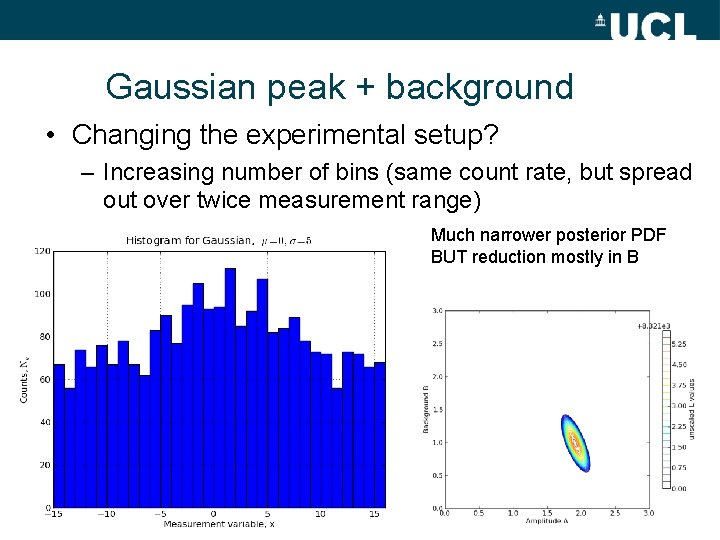
Gaussian peak + background • Changing the experimental setup? – Increasing number of bins (same count rate, but spread out over twice measurement range) Much narrower posterior PDF BUT reduction mostly in B

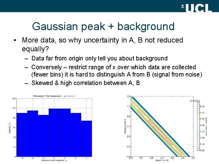
Gaussian peak + background • More data, so why uncertainty in A, B not reduced equally? – Data far from origin only tell you about background – Conversely – restrict range of x over which data are collected (fewer bins) it is hard to distinguish A from B (signal from noise) – Skewed & high correlation between A, B

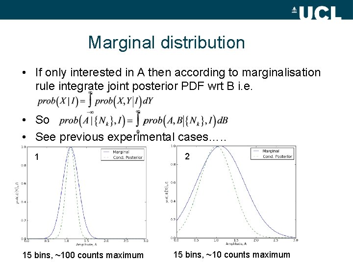
Marginal distribution • If only interested in A then according to marginalisation rule integrate joint posterior PDF wrt B i. e. • So • See previous experimental cases…. . 1 15 bins, ~100 counts maximum 2 15 bins, ~10 counts maximum

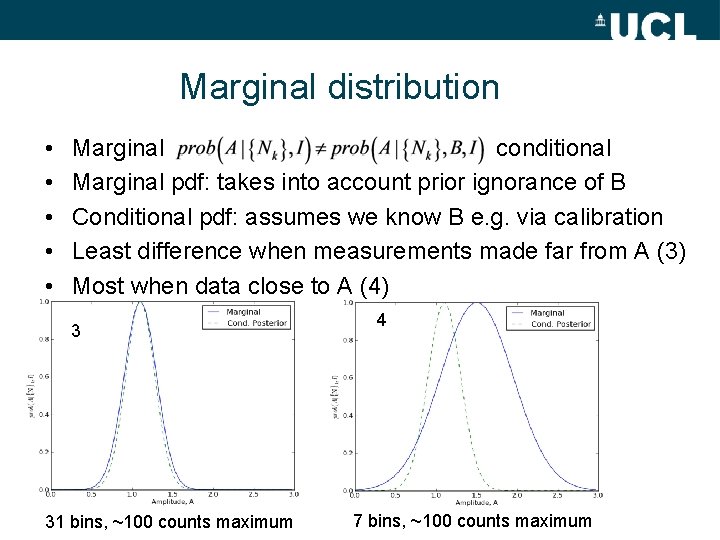
Marginal distribution • • • Marginal conditional Marginal pdf: takes into account prior ignorance of B Conditional pdf: assumes we know B e. g. via calibration Least difference when measurements made far from A (3) Most when data close to A (4) 3 31 bins, ~100 counts maximum 4 7 bins, ~100 counts maximum

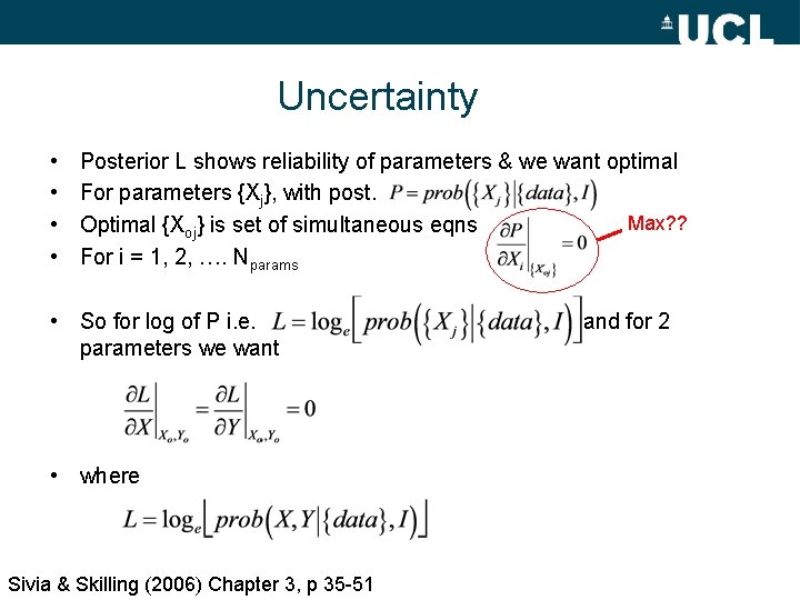
Uncertainty • • Posterior L shows reliability of parameters & we want optimal For parameters {Xj}, with post. Max? ? Optimal {Xoj} is set of simultaneous eqns For i = 1, 2, …. Nparams • So for log of P i. e. parameters we want • where Sivia & Skilling (2006) Chapter 3, p 35 -51 and for 2

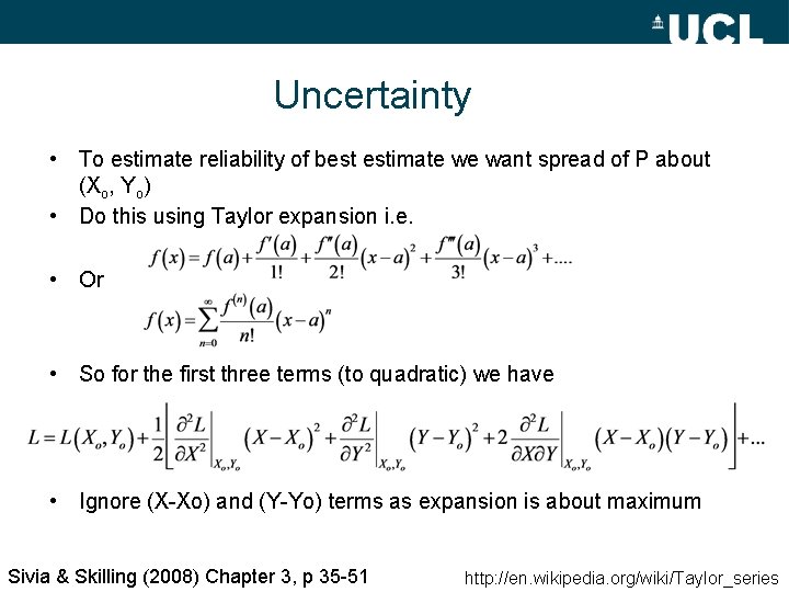
Uncertainty • To estimate reliability of best estimate we want spread of P about (Xo, Yo) • Do this using Taylor expansion i. e. • Or • So for the first three terms (to quadratic) we have • Ignore (X-Xo) and (Y-Yo) terms as expansion is about maximum Sivia & Skilling (2008) Chapter 3, p 35 -51 http: //en. wikipedia. org/wiki/Taylor_series

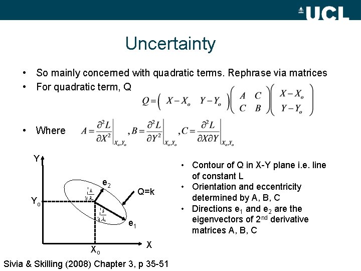
Uncertainty • So mainly concerned with quadratic terms. Rephrase via matrices • For quadratic term, Q • Where Y e 2 Q=k Yo e 1 Xo X Sivia & Skilling (2008) Chapter 3, p 35 -51 • Contour of Q in X-Y plane i. e. line of constant L • Orientation and eccentricity determined by A, B, C • Directions e 1 and e 2 are the eigenvectors of 2 nd derivative matrices A, B, C

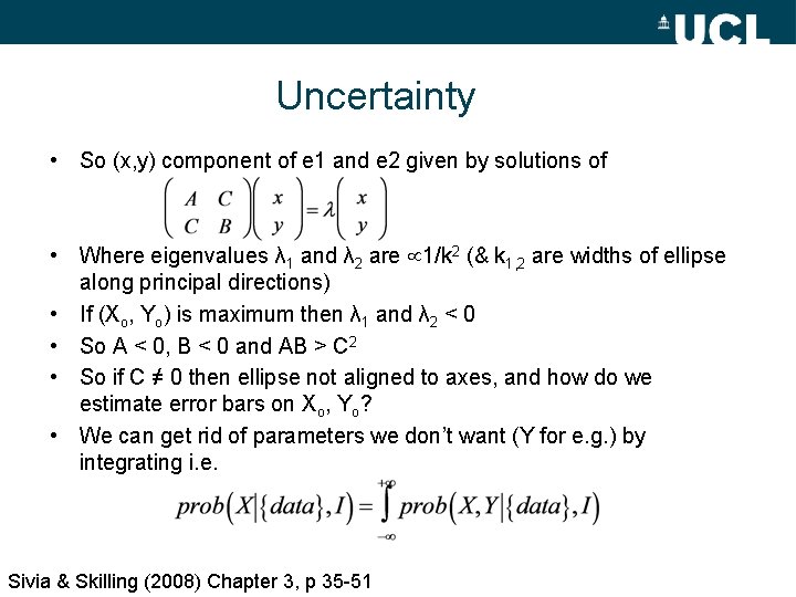
Uncertainty • So (x, y) component of e 1 and e 2 given by solutions of • Where eigenvalues λ 1 and λ 2 are 1/k 2 (& k 1, 2 are widths of ellipse along principal directions) • If (Xo, Yo) is maximum then λ 1 and λ 2 < 0 • So A < 0, B < 0 and AB > C 2 • So if C ≠ 0 then ellipse not aligned to axes, and how do we estimate error bars on Xo, Yo? • We can get rid of parameters we don’t want (Y for e. g. ) by integrating i. e. Sivia & Skilling (2008) Chapter 3, p 35 -51

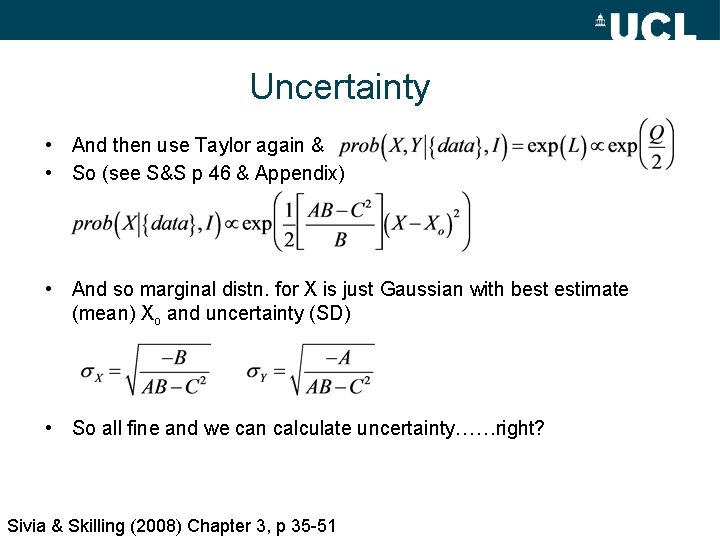
Uncertainty • And then use Taylor again & • So (see S&S p 46 & Appendix) • And so marginal distn. for X is just Gaussian with best estimate (mean) Xo and uncertainty (SD) • So all fine and we can calculate uncertainty……right? Sivia & Skilling (2008) Chapter 3, p 35 -51

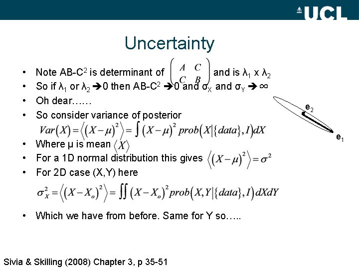
Uncertainty • • Note AB-C 2 is determinant of and is λ 1 x λ 2 So if λ 1 or λ 2 0 then AB-C 2 0 and σX and σY ∞ Oh dear…… So consider variance of posterior • Where μ is mean • For a 1 D normal distribution this gives • For 2 D case (X, Y) here • Which we have from before. Same for Y so…. . Sivia & Skilling (2008) Chapter 3, p 35 -51 e 2 e 1

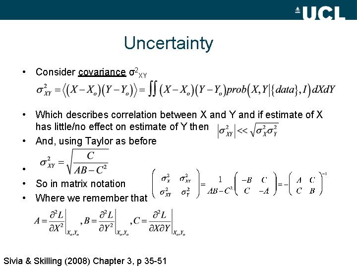
Uncertainty • Consider covariance σ2 XY • Which describes correlation between X and Y and if estimate of X has little/no effect on estimate of Y then • And, using Taylor as before • • So in matrix notation • Where we remember that Sivia & Skilling (2008) Chapter 3, p 35 -51

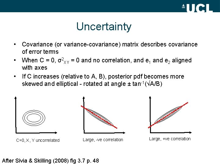
Uncertainty • Covariance (or variance-covariance) matrix describes covariance of error terms • When C = 0, σ2 XY = 0 and no correlation, and e 1 and e 2 aligned with axes • If C increases (relative to A, B), posterior pdf becomes more skewed and elliptical - rotated at angle ± tan-1(√A/B) C=0, X, Y uncorrelated Large, -ve correlation After Sivia & Skilling (2008) fig 3. 7 p. 48 Large, +ve correlation

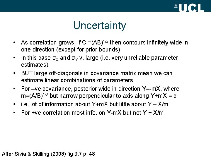
Uncertainty • As correlation grows, if C =(AB)1/2 then contours infinitely wide in one direction (except for prior bounds) • In this case σX and σY v. large (i. e. very unreliable parameter estimates) • BUT large off-diagonals in covariance matrix mean we can estimate linear combinations of parameters • For –ve covariance, posterior wide in direction Y=-m. X, where m=(A/B)1/2 but narrow perpendicular to axis along Y+m. X = c • i. e. lot of information about Y+m. X but little about Y – X/m • For +ve correlation most info. on Y-m. X but not Y + X/m After Sivia & Skilling (2008) fig 3. 7 p. 48

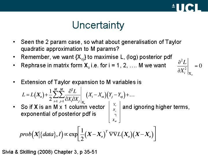
Uncertainty • Seen the 2 param case, so what about generalisation of Taylor quadratic approximation to M params? • Remember, we want {Xoj} to maximise L, (log) posterior pdf • Rephrase in matrix form Xo i. e. for i = 1, 2, …. M we want • Extension of Taylor expansion to M variables is • So if X is an M x 1 column vector exponential of posterior pdf is Sivia & Skilling (2008) Chapter 3, p 35 -51 and ignoring higher terms,

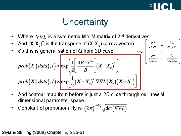
Uncertainty • Where is a symmetric M x M matrix of 2 nd derivatives • And (X-Xo)T is the transpose of (X-Xo) (a row vector) • So this is generalisation of Q from 2 D case • And contour map from before is just a 2 D slice through our now M dimensional parameter space • Constant of proportionality is Sivia & Skilling (2008) Chapter 3, p 35 -51

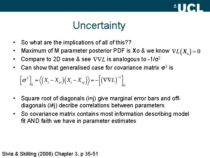
Uncertainty • • So what are the implications of all of this? ? Maximum of M parameter posterior PDF is Xo & we know Compare to 2 D case & see is analogous to -1/σ2 Can show that generalised case for covariance matrix σ2 is • Square root of diagonals (i=j) give marginal error bars and offdiagonals (i≠j) decribe correlations between parameters • So covariance matrix contains most information describing model fit AND faith we have in parameter estimates Sivia & Skilling (2008) Chapter 3, p 35 -51

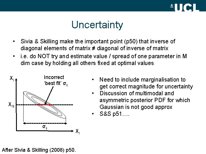
Uncertainty • Sivia & Skilling make the important point (p 50) that inverse of diagonal elements of matrix ≠ diagonal of inverse of matrix • i. e. do NOT try and estimate value / spread of one parameter in M dim case by holding all others fixed at optimal values Xj Incorrect ‘best fit’ σii • Need to include marginalisation to get correct magnitude for uncertainty • Discussion of multimodal and asymmetric posterior PDF for which Gaussian is not good approx • S&S p 51…. Xoj σii Xi After Sivia & Skilling (2008) p 50.

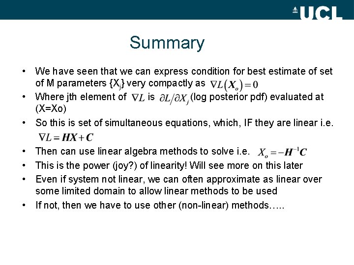
Summary • We have seen that we can express condition for best estimate of set of M parameters {Xj} very compactly as • Where jth element of is (log posterior pdf) evaluated at (X=Xo) • So this is set of simultaneous equations, which, IF they are linear i. e. • Then can use linear algebra methods to solve i. e. • This is the power (joy? ) of linearity! Will see more on this later • Even if system not linear, we can often approximate as linear over some limited domain to allow linear methods to be used • If not, then we have to use other (non-linear) methods…. .

Summary • Two parameter eg: Gaussian peak + background • Solve via Bayes’ T using Taylor expansion (to quadratic) • Issues over experimental setup – Integration time, number of bins, size etc. – Impact on posterior PDF • Can use linear methods to derive uncertainty estimates and explore correlation between parameters • Extend to multi-dimensional case using same method • Be careful when dealing with uncertainty • KEY: not always useful to look for summary statistics – if in doubt look at the posterior PDF – this gives full description