Motion Wed April 20 Kristen Grauman UTAustin Many

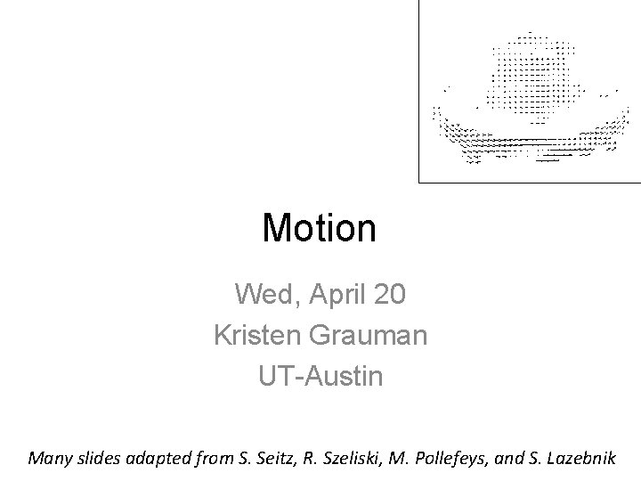
Motion Wed, April 20 Kristen Grauman UT-Austin Many slides adapted from S. Seitz, R. Szeliski, M. Pollefeys, and S. Lazebnik

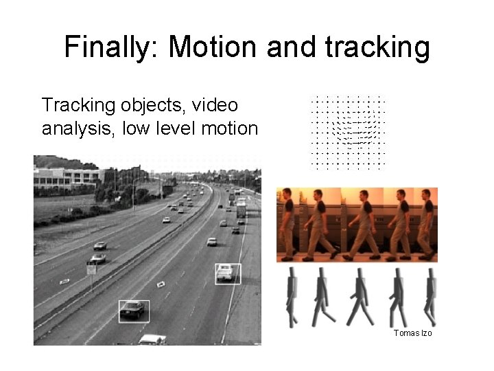
Finally: Motion and tracking Tracking objects, video analysis, low level motion Tomas Izo

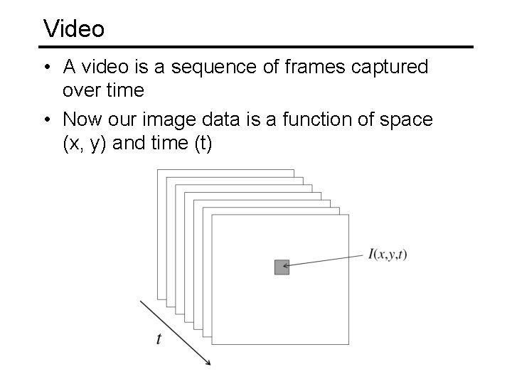
Video • A video is a sequence of frames captured over time • Now our image data is a function of space (x, y) and time (t)

Uses of motion • • • Estimating 3 D structure Segmenting objects based on motion cues Learning dynamical models Recognizing events and activities Improving video quality (motion stabilization)

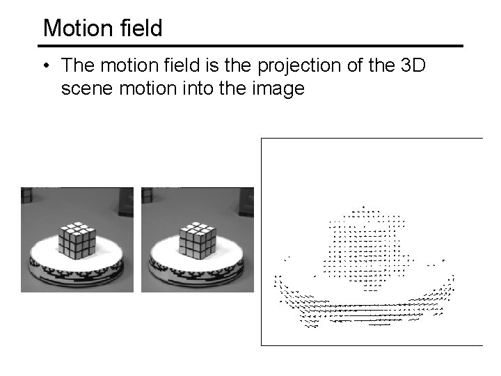
Motion field • The motion field is the projection of the 3 D scene motion into the image

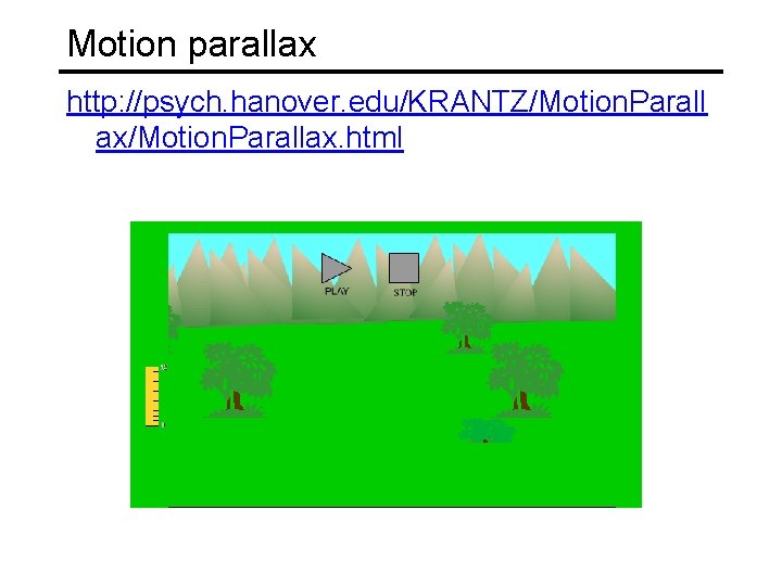
Motion parallax http: //psych. hanover. edu/KRANTZ/Motion. Parall ax/Motion. Parallax. html

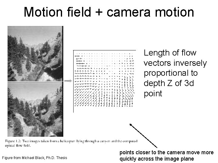
Motion field + camera motion Length of flow vectors inversely proportional to depth Z of 3 d point Figure from Michael Black, Ph. D. Thesis points closer to the camera move more quickly across the image plane

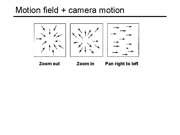
Motion field + camera motion Zoom out Zoom in Pan right to left

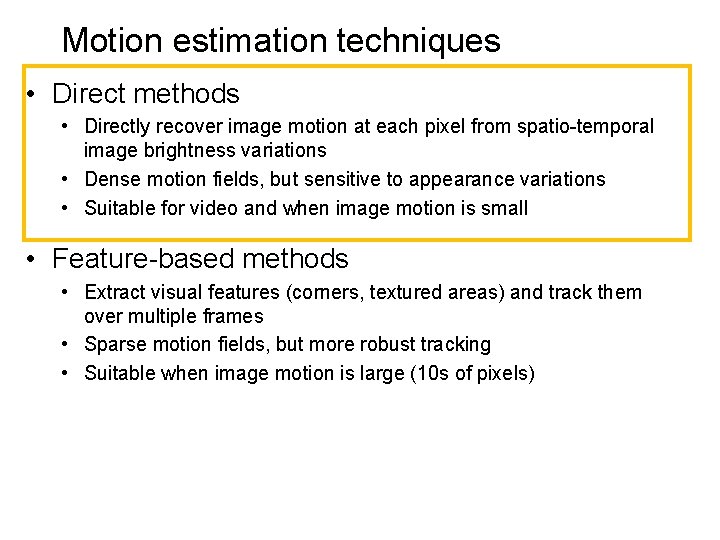
Motion estimation techniques • Direct methods • Directly recover image motion at each pixel from spatio-temporal image brightness variations • Dense motion fields, but sensitive to appearance variations • Suitable for video and when image motion is small • Feature-based methods • Extract visual features (corners, textured areas) and track them over multiple frames • Sparse motion fields, but more robust tracking • Suitable when image motion is large (10 s of pixels)

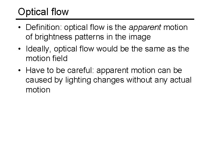
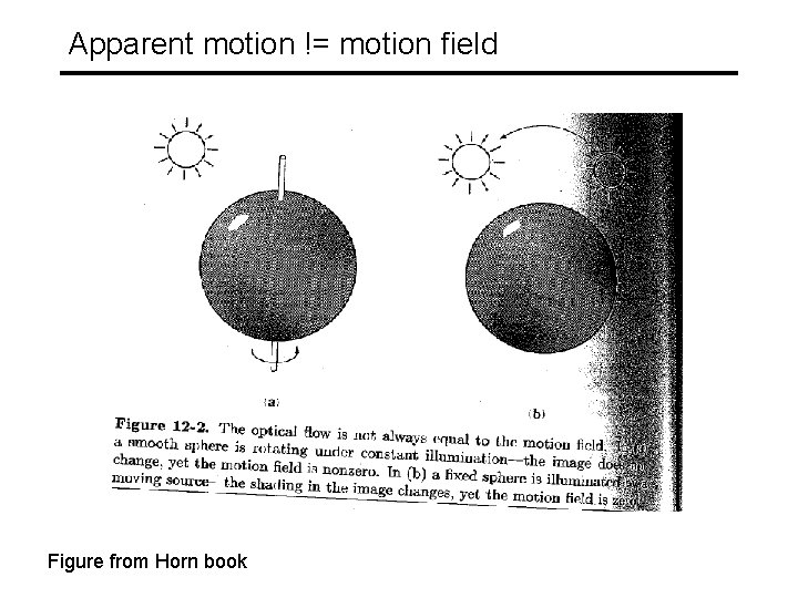
Optical flow • Definition: optical flow is the apparent motion of brightness patterns in the image • Ideally, optical flow would be the same as the motion field • Have to be careful: apparent motion can be caused by lighting changes without any actual motion

Apparent motion != motion field Figure from Horn book

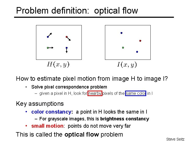
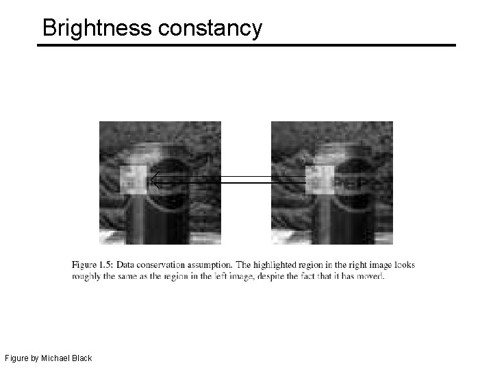
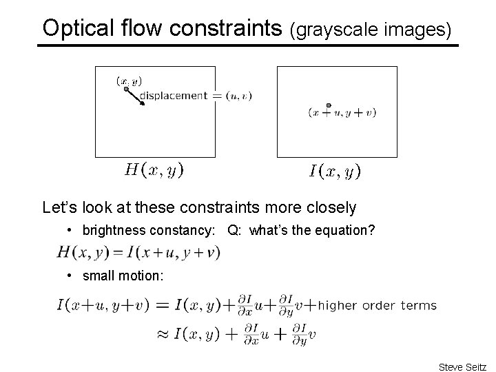
Problem definition: optical flow How to estimate pixel motion from image H to image I? • Solve pixel correspondence problem – given a pixel in H, look for nearby pixels of the same color in I Key assumptions • color constancy: a point in H looks the same in I – For grayscale images, this is brightness constancy • small motion: points do not move very far This is called the optical flow problem Steve Seitz

Brightness constancy Figure by Michael Black

Optical flow constraints (grayscale images) Let’s look at these constraints more closely • brightness constancy: Q: what’s the equation? • small motion: Steve Seitz

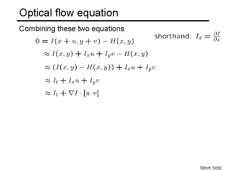
Optical flow equation Combining these two equations Steve Seitz

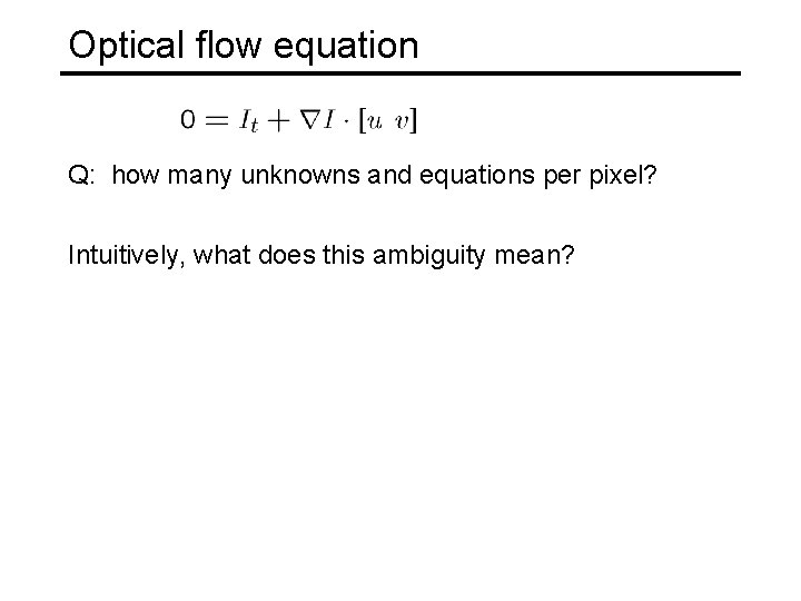
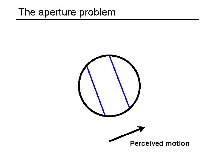
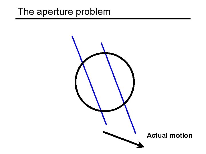
Optical flow equation Q: how many unknowns and equations per pixel? Intuitively, what does this ambiguity mean?

The aperture problem Perceived motion

The aperture problem Actual motion

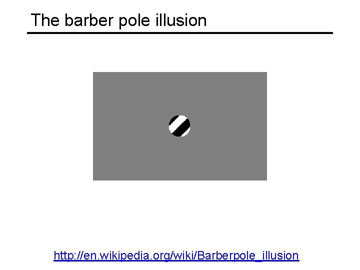
The barber pole illusion http: //en. wikipedia. org/wiki/Barberpole_illusion

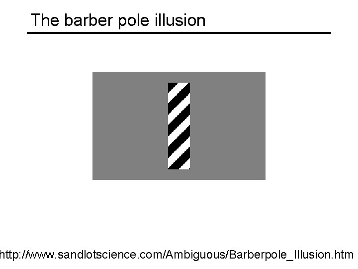
The barber pole illusion http: //www. sandlotscience. com/Ambiguous/Barberpole_Illusion. htm

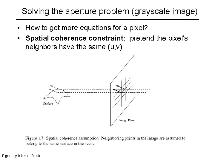
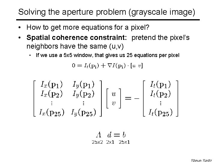
Solving the aperture problem (grayscale image) • How to get more equations for a pixel? • Spatial coherence constraint: pretend the pixel’s neighbors have the same (u, v) Figure by Michael Black

Solving the aperture problem (grayscale image) • How to get more equations for a pixel? • Spatial coherence constraint: pretend the pixel’s neighbors have the same (u, v) • If we use a 5 x 5 window, that gives us 25 equations per pixel

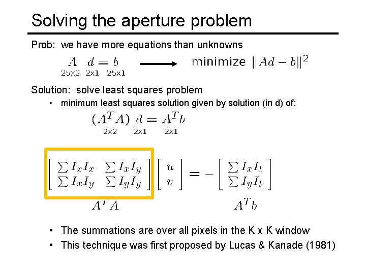
Solving the aperture problem Prob: we have more equations than unknowns Solution: solve least squares problem • minimum least squares solution given by solution (in d) of: • The summations are over all pixels in the K x K window • This technique was first proposed by Lucas & Kanade (1981)

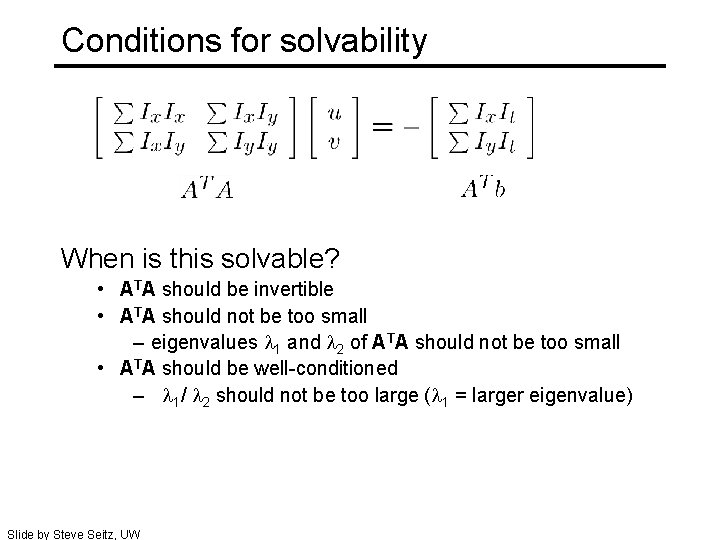
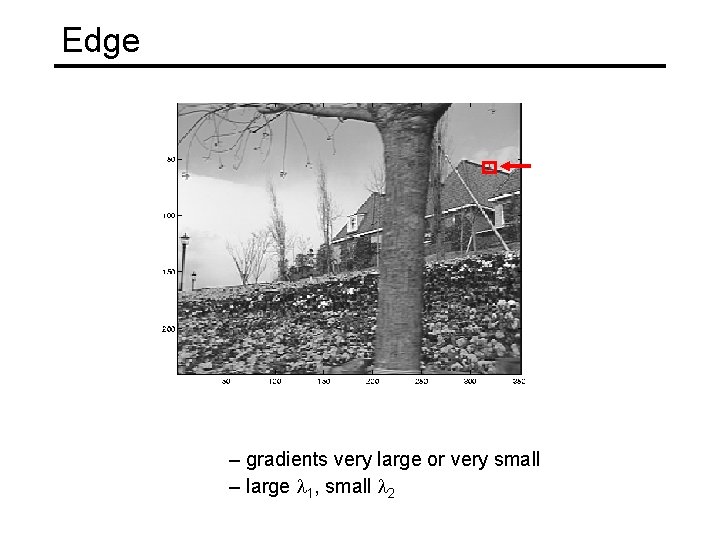
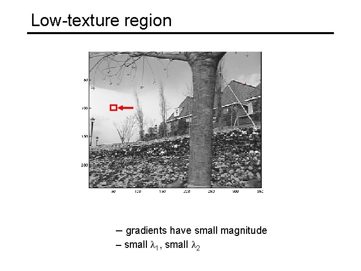
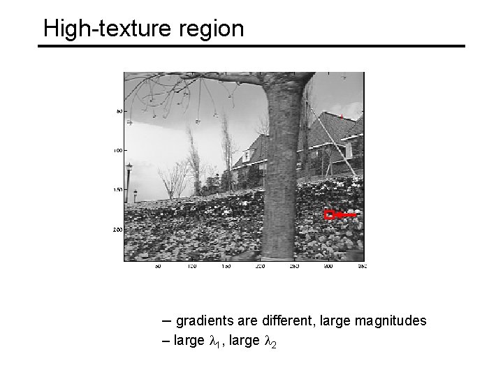
Conditions for solvability When is this solvable? • ATA should be invertible • ATA should not be too small – eigenvalues l 1 and l 2 of ATA should not be too small • ATA should be well-conditioned – l 1/ l 2 should not be too large (l 1 = larger eigenvalue) Slide by Steve Seitz, UW

Edge – gradients very large or very small – large l 1, small l 2

Low-texture region – gradients have small magnitude – small l 1, small l 2

High-texture region – gradients are different, large magnitudes – large l 1, large l 2

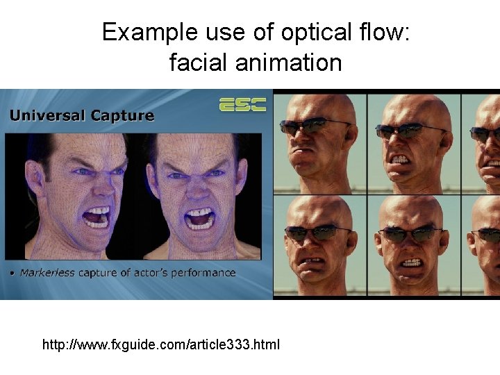
Example use of optical flow: facial animation http: //www. fxguide. com/article 333. html

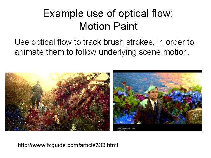
Example use of optical flow: Motion Paint Use optical flow to track brush strokes, in order to animate them to follow underlying scene motion. http: //www. fxguide. com/article 333. html

Fun with flow • http: //www. youtube. com/watch? v=Tb. Jrc 6 QCe. U 0&feature=related • http: //www. youtube. com/watch? v=pck. Facs IWg 4

Motion vs. Stereo: Similarities • Both involve solving – Correspondence: disparities, motion vectors – Reconstruction

Motion vs. Stereo: Differences • Motion: – Uses velocity: consecutive frames must be close to get good approximate time derivative – 3 d movement between camera and scene not necessarily single 3 d rigid transformation • Whereas with stereo: – Could have any disparity value – View pair separated by a single 3 d transformation

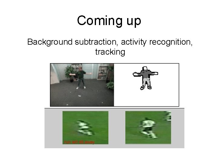
Coming up Background subtraction, activity recognition, tracking