Modeling and Segmentation of Dynamic Textures Atiyeh Ghoreyshi

Modeling and Segmentation of Dynamic Textures Atiyeh Ghoreyshi, Avinash Ravichandran, René Vidal Center for Imaging Science Institute for Computational Medicine Johns Hopkins University

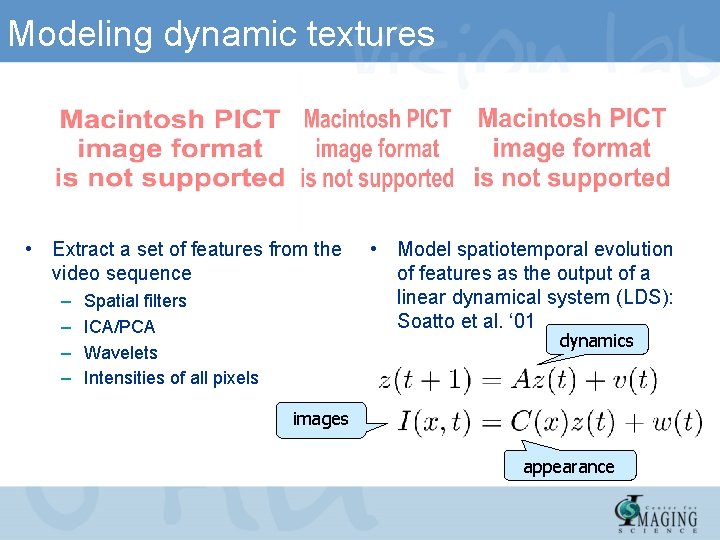
Modeling dynamic textures • Extract a set of features from the video sequence – – Spatial filters ICA/PCA Wavelets Intensities of all pixels • Model spatiotemporal evolution of features as the output of a linear dynamical system (LDS): Soatto et al. ‘ 01 dynamics images appearance

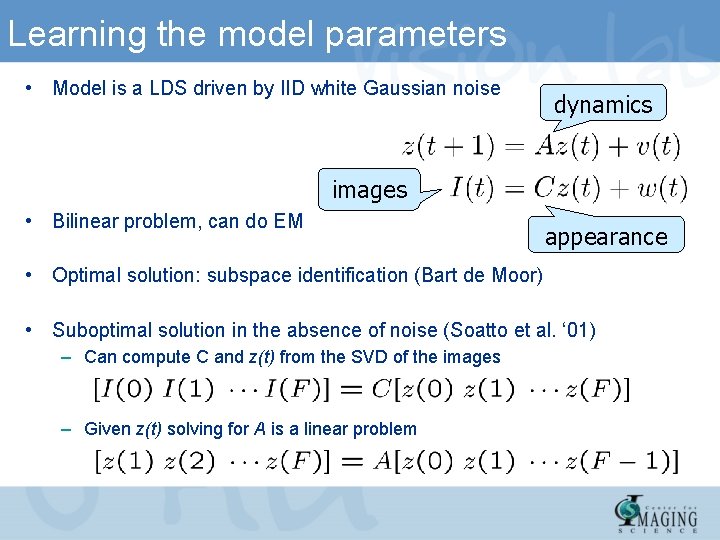
Learning the model parameters • Model is a LDS driven by IID white Gaussian noise dynamics images • Bilinear problem, can do EM appearance • Optimal solution: subspace identification (Bart de Moor) • Suboptimal solution in the absence of noise (Soatto et al. ‘ 01) – Can compute C and z(t) from the SVD of the images – Given z(t) solving for A is a linear problem

Synthesizing novel sequences • Once a model of a dynamic texture has been learned, one can use it to synthesize novel sequences: – Shöld et al. ’ 00, Soatto et al. ’ 01, Doretto et al. ’ 03, Yuan et al. ‘ 04

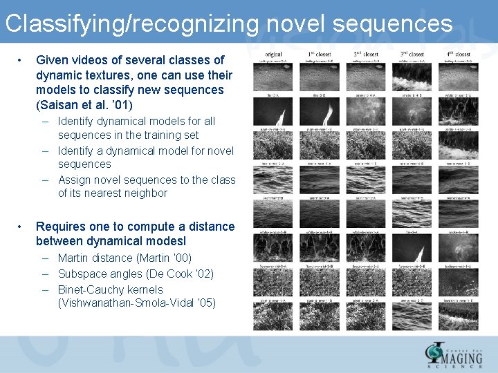
Classifying/recognizing novel sequences • Given videos of several classes of dynamic textures, one can use their models to classify new sequences (Saisan et al. ’ 01) – Identify dynamical models for all sequences in the training set – Identify a dynamical model for novel sequences – Assign novel sequences to the class of its nearest neighbor • Requires one to compute a distance between dynamical modesl – Martin distance (Martin ’ 00) – Subspace angles (De Cook ‘ 02) – Binet-Cauchy kernels (Vishwanathan-Smola-Vidal ‘ 05)

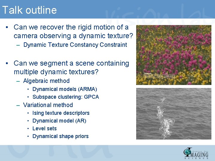
Talk outline • Can we recover the rigid motion of a camera observing a dynamic texture? – Dynamic Texture Constancy Constraint • Can we segment a scene containing multiple dynamic textures? – Algebraic method • Dynamical models (ARMA) • Subspace clustering: GPCA – Variational method • • Ising texture descriptors Dynamical model (AR) Level sets Dynamical shape priors

Part I Computing Optical Flow from Dynamic Textures Center for Imaging Science Institute for Computational Medicine Johns Hopkins University

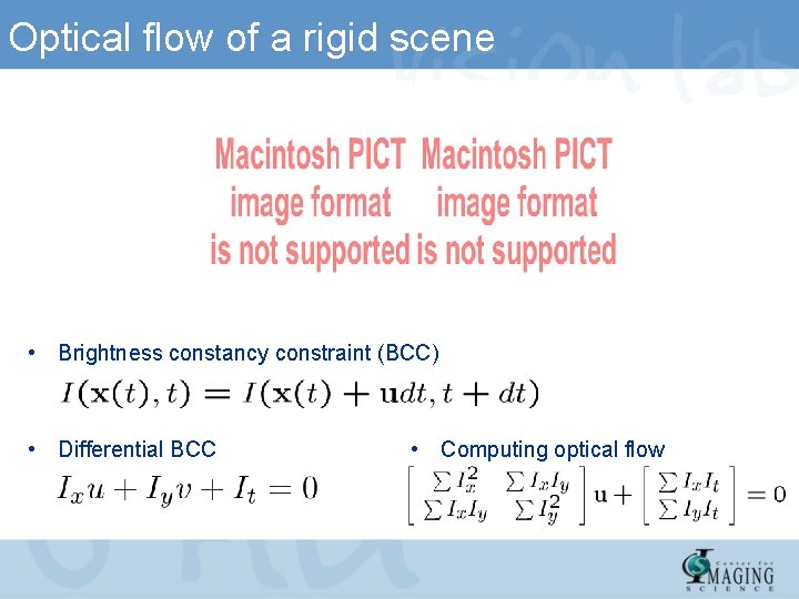
Optical flow of a rigid scene • Brightness constancy constraint (BCC) • Differential BCC • Computing optical flow

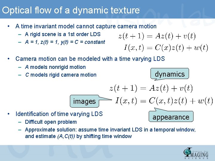
Optical flow of a dynamic texture • A time invariant model cannot capture camera motion – A rigid scene is a 1 st order LDS – A = 1, z(t) = 1, y(t) = C = constant • Camera motion can be modeled with a time varying LDS – A models nonrigid motion – C models rigid camera motion dynamics images • Identification of time varying LDS appearance – Difficult open problem – Approximate solution: assume time invariant LDS in a temporal window, and estimate (A, C(t)) by shifting time window

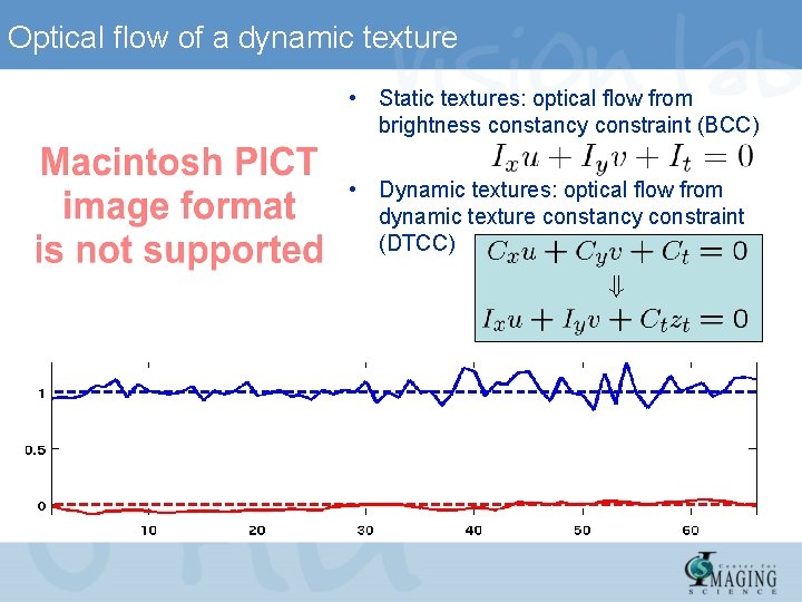
Optical flow of a dynamic texture • Static textures: optical flow from brightness constancy constraint (BCC) • Dynamic textures: optical flow from dynamic texture constancy constraint (DTCC)

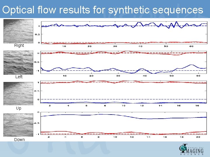
Optical flow results for synthetic sequences Right Left Up Down

Optical flow of flowerbed sequence

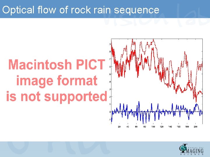
Optical flow of rock rain sequence

Part II Segmentation Dynamic Textures Atiyeh Ghoreyshi Center for Imaging Science Institute for Computational Medicine Johns Hopkins University

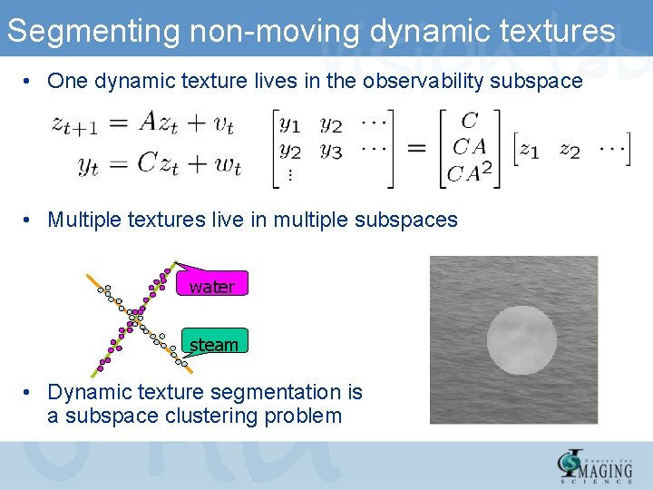
Segmenting non-moving dynamic textures • One dynamic texture lives in the observability subspace • Multiple textures live in multiple subspaces water steam • Dynamic texture segmentation is a subspace clustering problem

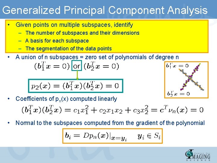
Generalized Principal Component Analysis • Given points on multiple subspaces, identify – The number of subspaces and their dimensions – A basis for each subspace – The segmentation of the data points • A union of n subspaces = zero set of polynomials of degree n • Coefficients of pn(x) computed linearly • Normal to the subspaces computed from the gradient of the polynomial

Segmenting water steam sequence • Multiple textures live in multiple subspaces water • Cluster the data using GPCA steam

Segmenting a cardiac-MR sequence • Goal: recognize multiple types of arrhythmias using heart MRI images • Model: visual dynamics are modeled as multiple dynamic textures – Heart motion: nonrigid – Chest motion: respiration

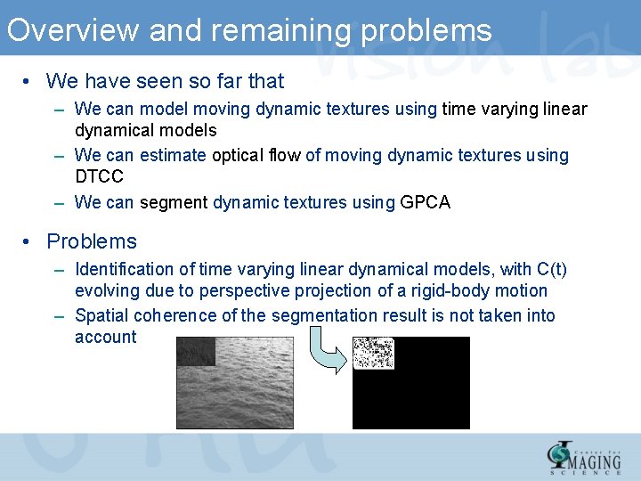
Overview and remaining problems • We have seen so far that – We can model moving dynamic textures using time varying linear dynamical models – We can estimate optical flow of moving dynamic textures using DTCC – We can segment dynamic textures using GPCA • Problems – Identification of time varying linear dynamical models, with C(t) evolving due to perspective projection of a rigid-body motion – Spatial coherence of the segmentation result is not taken into account

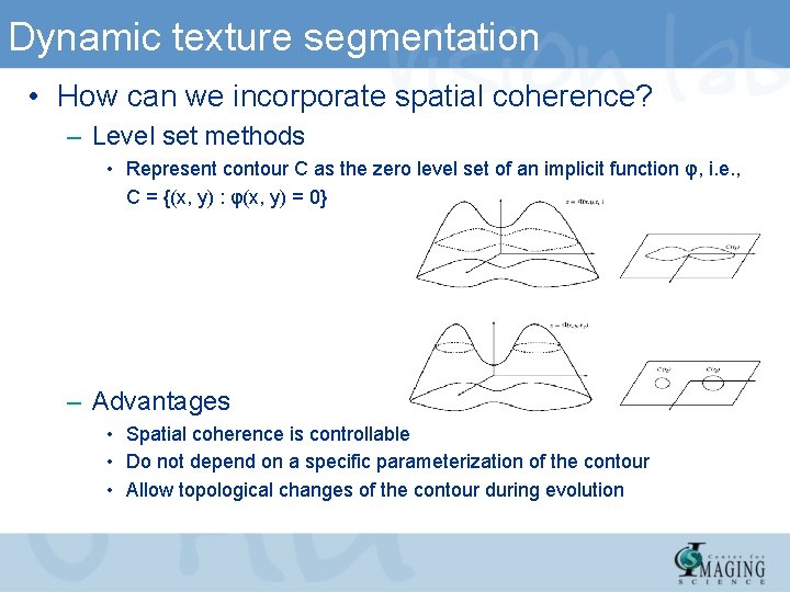
Dynamic texture segmentation • How can we incorporate spatial coherence? – Level set methods • Represent contour C as the zero level set of an implicit function φ, i. e. , C = {(x, y) : φ(x, y) = 0} – Advantages • Spatial coherence is controllable • Do not depend on a specific parameterization of the contour • Allow topological changes of the contour during evolution

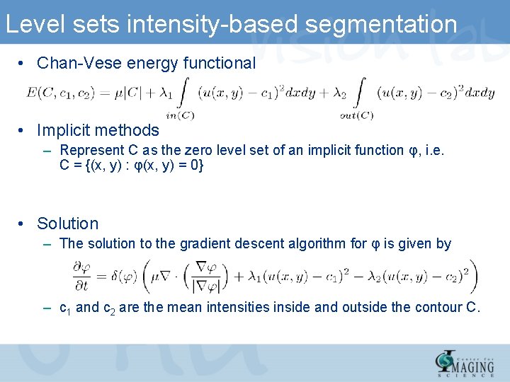
Level sets intensity-based segmentation • Chan-Vese energy functional • Implicit methods – Represent C as the zero level set of an implicit function φ, i. e. C = {(x, y) : φ(x, y) = 0} • Solution – The solution to the gradient descent algorithm for φ is given by – c 1 and c 2 are the mean intensities inside and outside the contour C.

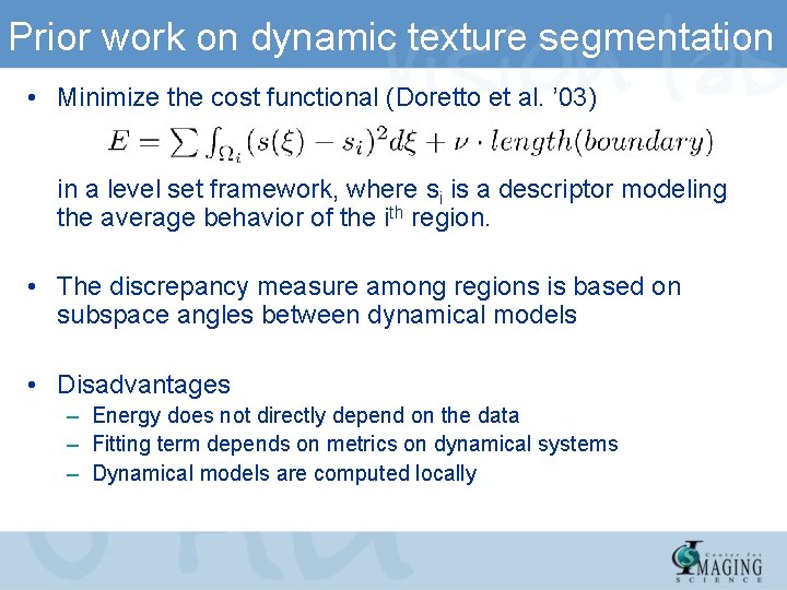
Prior work on dynamic texture segmentation • Minimize the cost functional (Doretto et al. ’ 03) in a level set framework, where si is a descriptor modeling the average behavior of the ith region. • The discrepancy measure among regions is based on subspace angles between dynamical models • Disadvantages – Energy does not directly depend on the data – Fitting term depends on metrics on dynamical systems – Dynamical models are computed locally

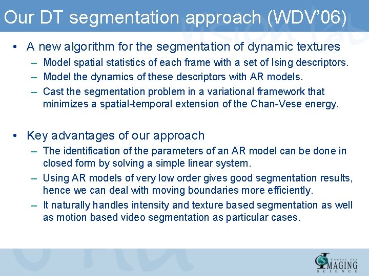
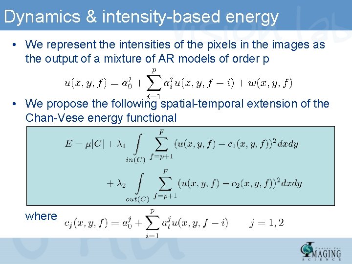
Our DT segmentation approach (WDV’ 06) • A new algorithm for the segmentation of dynamic textures – Model spatial statistics of each frame with a set of Ising descriptors. – Model the dynamics of these descriptors with AR models. – Cast the segmentation problem in a variational framework that minimizes a spatial-temporal extension of the Chan-Vese energy. • Key advantages of our approach – The identification of the parameters of an AR model can be done in closed form by solving a simple linear system. – Using AR models of very low order gives good segmentation results, hence we can deal with moving boundaries more efficiently. – It naturally handles intensity and texture based segmentation as well as motion based video segmentation as particular cases.

Dynamics & intensity-based energy • We represent the intensities of the pixels in the images as the output of a mixture of AR models of order p • We propose the following spatial-temporal extension of the Chan-Vese energy functional where

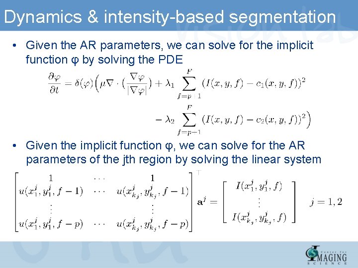
Dynamics & intensity-based segmentation • Given the AR parameters, we can solve for the implicit function φ by solving the PDE • Given the implicit function φ, we can solve for the AR parameters of the jth region by solving the linear system

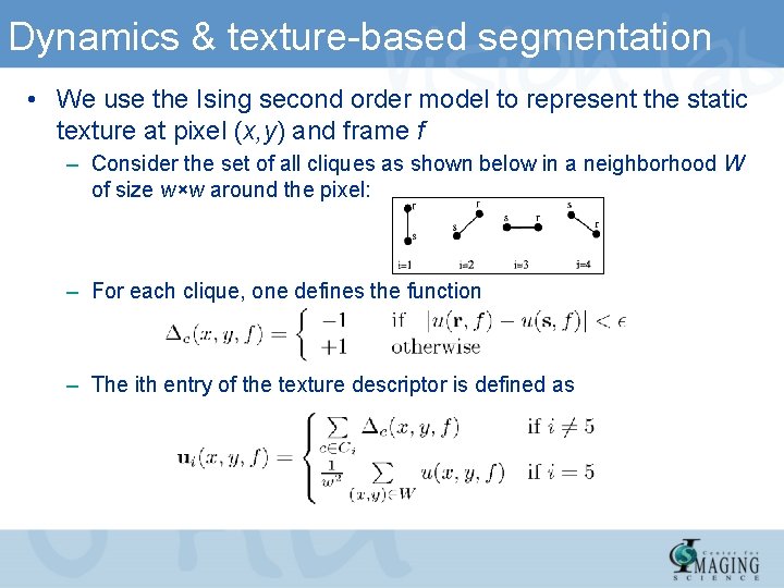
Dynamics & texture-based segmentation • We use the Ising second order model to represent the static texture at pixel (x, y) and frame f – Consider the set of all cliques as shown below in a neighborhood W of size w×w around the pixel: – For each clique, one defines the function – The ith entry of the texture descriptor is defined as

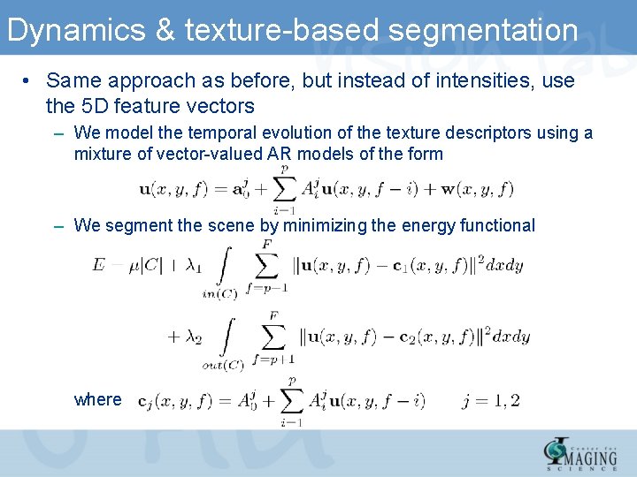
Dynamics & texture-based segmentation • Same approach as before, but instead of intensities, use the 5 D feature vectors – We model the temporal evolution of the texture descriptors using a mixture of vector-valued AR models of the form – We segment the scene by minimizing the energy functional where

Dynamics & texture-based segmentation • Alternating minimization method – Given the AR parameters, solve for the implicit function φ by solving the PDE. – Given the implicit function φ, solve for the AR parameters of the jth region by solving the linear system. • Implementation – Assume that the AR parameter matrices are diagonal. – Entries of the feature vector are outputs of five decoupled scalar AR models. – Can estimate the AR parameters independently for each entry of the texture descriptors, as we did before for the intensities.

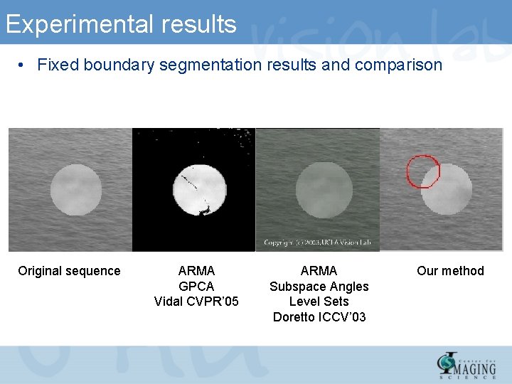
Experimental results • Fixed boundary segmentation results and comparison Original sequence ARMA GPCA Vidal CVPR’ 05 ARMA Subspace Angles Level Sets Doretto ICCV’ 03 Our method

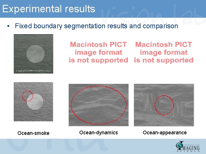
Experimental results • Fixed boundary segmentation results and comparison Ocean-smoke Ocean-dynamics Ocean-appearance

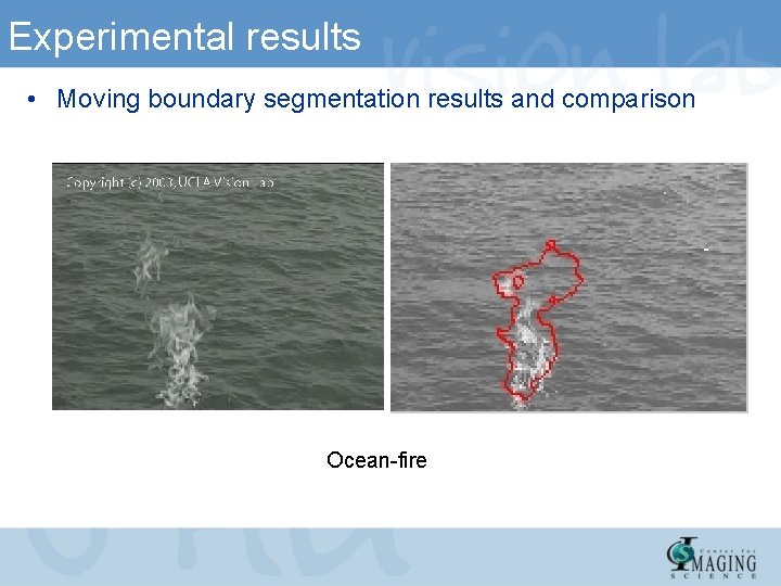
Experimental results • Moving boundary segmentation results and comparison Ocean-fire

Experimental results • Results on a real sequence Raccoon on River

Experimental Results • Segmentation of the epicardium One axial slice of a beating heart Segmentation results Initialized with GPCA

Conclusions • A new algorithm for the segmentation of dynamic textures – Model spatial statistics of each frame with a set of Ising descriptors – Model the dynamics of these descriptors with ARX models – Cast the segmentation problem in a variational framework that minimizes a spatial-temporal extension of the Chan-Vese energy • Key advantages of our approach – The identification of the parameters of an ARX model can be done in closed form by solving a simple linear system – Using ARX models of very low order gives good segmentation results, hence we can deal with moving boundaries more efficiently – It naturally handles intensity and texture based segmentation as well as motion based video segmentation as particular cases

Overview and remaining problems • So far, we have – Modeled moving and non-moving dynamic textures – Estimated optical flow of moving dynamic textures – Segmented dynamic textures • We have yet to – Improve the accuracy of the results for more sensitive settings such as medical image segmentation. – Improve the robustness to • Initialization • Noise • Low resolution data

Segmentation using priors • One solution could be incorporating prior knowledge about the attributes of our region of interest. • Previous work – Priors on shape • Tsai et al. ’ 03, Kaus et al. ’ 03, Pluempitiwiriyawej et al. ’ 05 • Model-based segmentation: Horkaew and Yang ’ 03, Biechel et al. ‘ 05 – Priors on shape and intensity • Rousson and Cremers ‘ 05

Dynamic texture segmentation using priors • We propose a new algorithm for the segmentation of dynamic scenes using priors on shape, intensity, and AR parameters 1. Represent manually segmented training images by their signed distance functions. 2. Registration within the training set, followed by PCA on the space of signed distance functions. 3. Model the dynamics of the regions with AR models; build pdf’s of the AR parameters and intensity for each region using histograms. 4. Maximize a log-likelihood function using level set methods.

Shape variability • A two level approach: 1. Align the true masks using similarity transformations 2. Extract the remaining variability by using PCA on the space of signed distance functions 1. Registration using gradient descent on the energy functional with respect to translation, rotation, and scale. • PCA on the matrix , where each column is a columnized signed distance function corresponding to a shape in the training set.

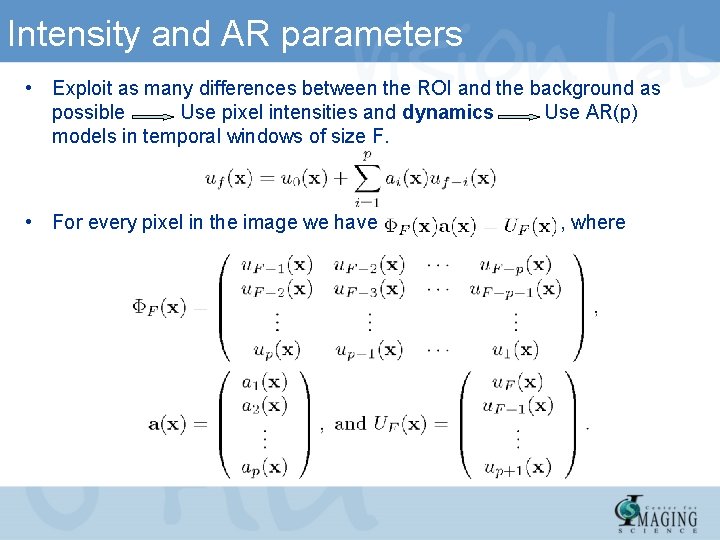
Intensity and AR parameters • Exploit as many differences between the ROI and the background as possible Use pixel intensities and dynamics Use AR(p) models in temporal windows of size F. • For every pixel in the image we have , where

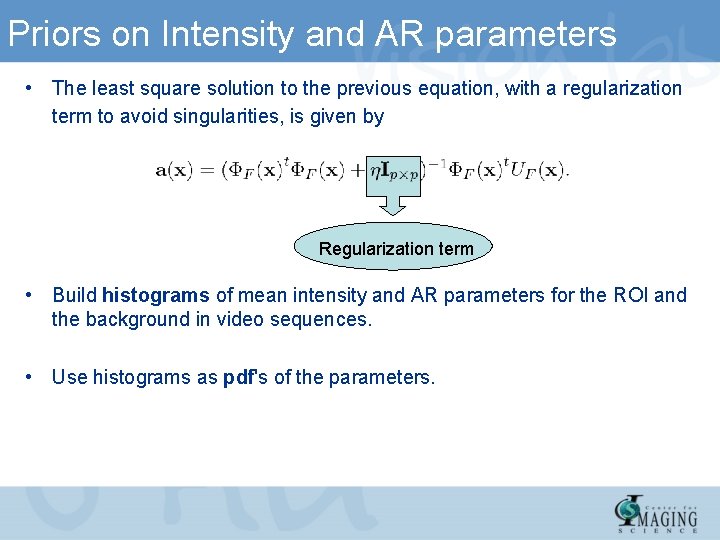
Priors on Intensity and AR parameters • The least square solution to the previous equation, with a regularization term to avoid singularities, is given by Regularization term • Build histograms of mean intensity and AR parameters for the ROI and the background in video sequences. • Use histograms as pdf's of the parameters.

Segmentation using ML and level sets • Find the parameters that maximize the log-likelihood function • Which is equivalent to minimizing where φ and H(φ) are the current signed distance and heaviside functions, and Pin and Pout are the joint pdf of the intensity and AR parameters for the ROI and the background respectively. • Minimize EML using a gradient descent algorithm with respect to the pose parameters and the weights of the shape principal components.

Experimental Results • For our experiments, we use a dataset containing 7 video sequences corresponding to 7 axial slices of the heart. Each video sequence is composed of 30 frames of size 128 x 128 spanning over one complete beating cycle. We use AR(2) models with temporal windows of size 5. • Registration Results Unregistered mean training shape Registered mean training shape

Histograms of intensity and AR parameters • We calculate the joint pdf of the variables as the product of their individual pdf's, assuming independence. a 1 histograms a 2 histograms Intensity histograms Top: Heart Bottom: Background

Segmentation Results First slice Green: Initialization Red: Final segmentation Seventh slice

Comparison • Statistics of Epicardium Segmentation Results with and without AR parameter priors

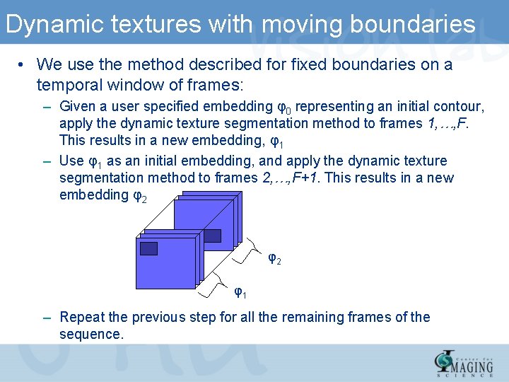
Dynamic textures with moving boundaries • We use the method described for fixed boundaries on a temporal window of frames: – Given a user specified embedding φ0 representing an initial contour, apply the dynamic texture segmentation method to frames 1, …, F. This results in a new embedding, φ1 – Use φ1 as an initial embedding, and apply the dynamic texture segmentation method to frames 2, …, F+1. This results in a new embedding φ2 φ2 φ1 – Repeat the previous step for all the remaining frames of the sequence.