Maintaining Variance and kMedians over Data Stream Windows

Maintaining Variance and k-Medians over Data Stream Windows Brian Babcock, Mayur Datar, Rajeev Motwani, Liadan O’Callaghan Stanford University

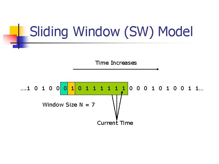
Data Streams and Sliding Windows n Streaming data model n n Useful for applications with high data volumes, timeliness requirements Data processed in single pass Limited memory (sublinear in stream size) Sliding window model n n Variation of streaming data model Only recent data matters Parameterized by window size N Limited memory (sublinear in window size)

Sliding Window (SW) Model Time Increases …. 1 0 0 0 1 1 1 1 0 0 0 1 1… Window Size N = 7 Current Time

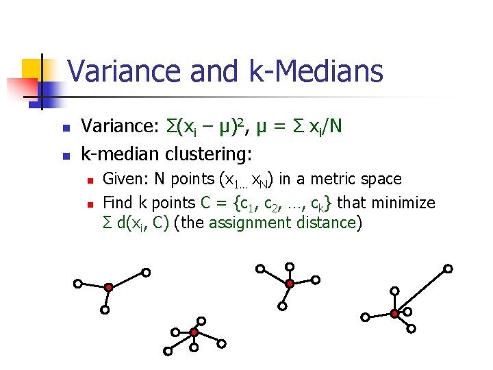
Variance and k-Medians n n Variance: Σ(xi – μ)2, μ = Σ xi/N k-median clustering: n n Given: N points (x 1… x. N) in a metric space Find k points C = {c 1, c 2, …, ck} that minimize Σ d(xi, C) (the assignment distance)

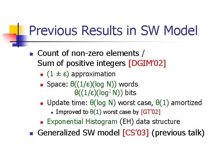
Previous Results in SW Model n Count of non-zero elements / Sum of positive integers [DGIM’ 02] n n n (1 ± ε) approximation Space: θ((1/ε)(log N)) words θ((1/ε)(log 2 N)) bits Update time: θ(log N) worst case, θ(1) amortized n n n Improved to θ(1) worst case by [GT’ 02] Exponential Histogram (EH) data structure Generalized SW model [CS’ 03] (previous talk)

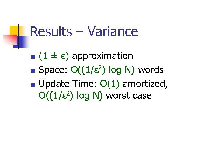
Results – Variance n n n (1 ± ε) approximation Space: O((1/ε 2) log N) words Update Time: O(1) amortized, O((1/ε 2) log N) worst case

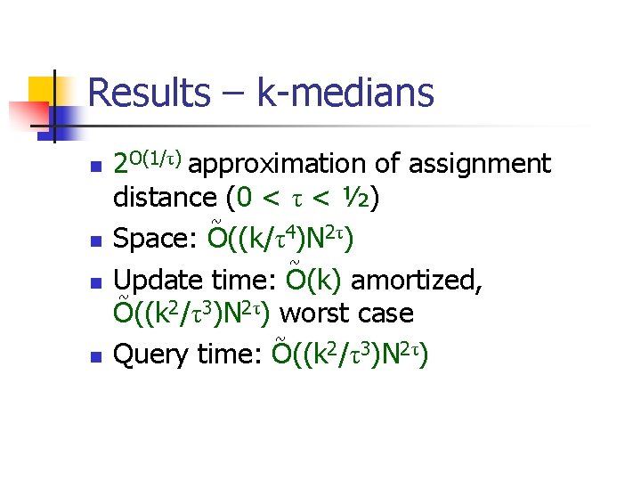
Results – k-medians n n 2 O(1/τ) approximation of assignment distance (0 < τ < ½) ~ Space: O((k/τ4)N 2τ) ~ Update time: O(k) amortized, ~ O((k 2/τ3)N 2τ) worst case ~ Query time: O((k 2/τ3)N 2τ)

Remainder of the Talk n n n Overview of Exponential Histogram Where EH fails and how to fix it Algorithm for Variance Main ideas in k-medians algorithm Open problems

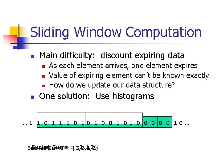
Sliding Window Computation n Main difficulty: discount expiring data n n As each element arrives, one element expires Value of expiring element can’t be known exactly How do we update our data structure? One solution: Use histograms …. 1 1 0 1 0 0 0 1 0 … Bucket. Sums=={3, 2, 1, 2} {2, 1, 2} Bucket

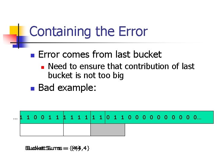
Containing the Error n Error comes from last bucket n n Need to ensure that contribution of last bucket is not too big Bad example: … 1 1 0 0 1 1 1 1 0 0 0 0 0… Bucket. Sums=={4, 4, 4} {4}

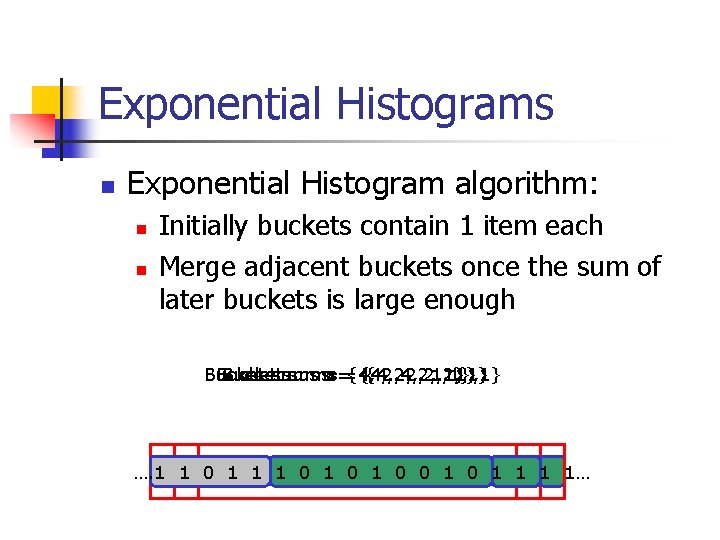
Exponential Histograms n Exponential Histogram algorithm: n n Initially buckets contain 1 item each Merge adjacent buckets once the sum of later buckets is large enough Bucket sums === {4, {4, 2, 2, 2, 1, 1} 2, 1} 1} 1 1} , 1} …. 1 1 0 1 0 1 0 1 1…

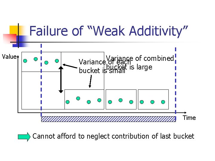
Where EH Goes Wrong n [DGIM’ 02] Can estimate any function f defined over windows that satisfies: n n n Positive: f(X) ≥ 0 Polynomially bounded: f(X) ≤ poly(|X|) Composable: Can compute f(X +Y) from f(X), f(Y) and little additional information Weakly Additive: (f(X) + f(Y)) ≤ f(X +Y) ≤ c(f(X) + f(Y)) “Weakly Additive” condition not valid for variance, k-medians

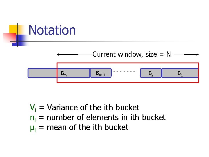
Notation Current window, size = N Bm Bm-1 ……………… B 2 Vi = Variance of the ith bucket ni = number of elements in ith bucket μi = mean of the ith bucket B 1

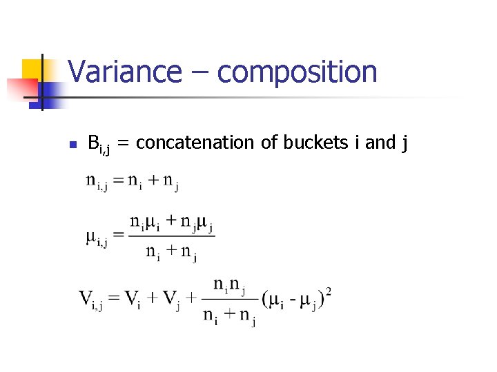
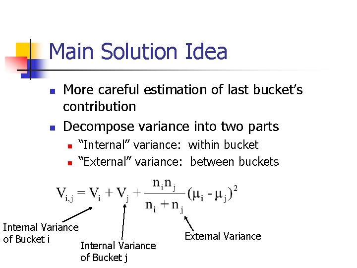
Variance – composition n Bi, j = concatenation of buckets i and j

Failure of “Weak Additivity” Value Variance of each of combined bucket isbucket small is large Time Cannot afford to neglect contribution of last bucket

Main Solution Idea n n More careful estimation of last bucket’s contribution Decompose variance into two parts n n Internal Variance of Bucket i “Internal” variance: within bucket “External” variance: between buckets Internal Variance of Bucket j External Variance

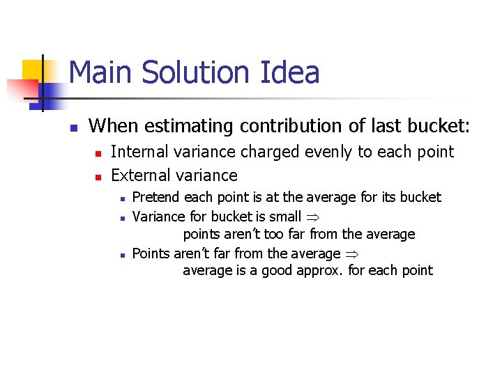
Main Solution Idea n When estimating contribution of last bucket: n n Internal variance charged evenly to each point External variance n n n Pretend each point is at the average for its bucket Variance for bucket is small points aren’t too far from the average Points aren’t far from the average is a good approx. for each point

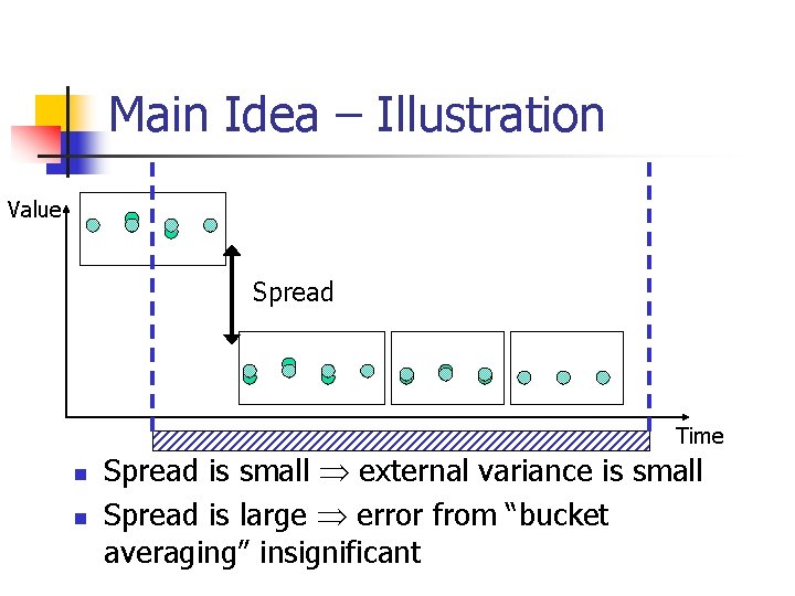
Main Idea – Illustration Value Spread Time n n Spread is small external variance is small Spread is large error from “bucket averaging” insignificant

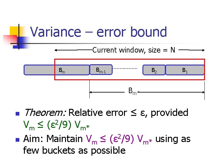
Variance – error bound Current window, size = N Bm Bm-1 ……………… B 2 B 1 Bm* n n Theorem: Relative error ≤ ε, provided Vm ≤ (ε 2/9) Vm* Aim: Maintain Vm ≤ (ε 2/9) Vm* using as few buckets as possible

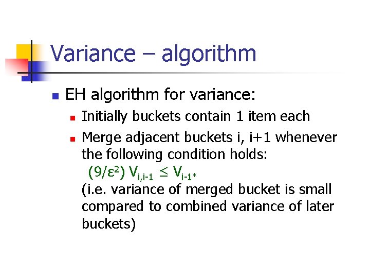
Variance – algorithm n EH algorithm for variance: n n Initially buckets contain 1 item each Merge adjacent buckets i, i+1 whenever the following condition holds: (9/ε 2) Vi, i-1 ≤ Vi-1* (i. e. variance of merged bucket is small compared to combined variance of later buckets)

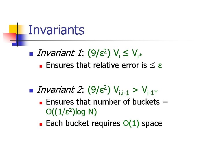
Invariants n Invariant 1: (9/ε 2) Vi ≤ Vi* n n Ensures that relative error is ≤ ε Invariant 2: (9/ε 2) Vi, i-1 > Vi-1* n n Ensures that number of buckets = O((1/ε 2)log N) Each bucket requires O(1) space

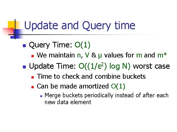
Update and Query time n Query Time: O(1) n n We maintain n, V & μ values for m and m* Update Time: O((1/ε 2) log N) worst case n n Time to check and combine buckets Can be made amortized O(1) n Merge buckets periodically instead of after each new data element

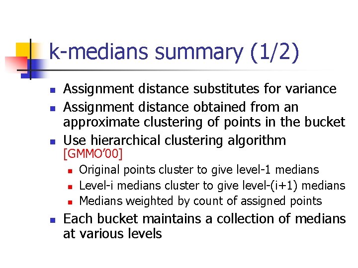
k-medians summary (1/2) n n Assignment distance substitutes for variance Assignment distance obtained from an approximate clustering of points in the bucket Use hierarchical clustering algorithm [GMMO’ 00] n Original points cluster to give level-1 medians n Level-i medians cluster to give level-(i+1) medians n Medians weighted by count of assigned points Each bucket maintains a collection of medians at various levels

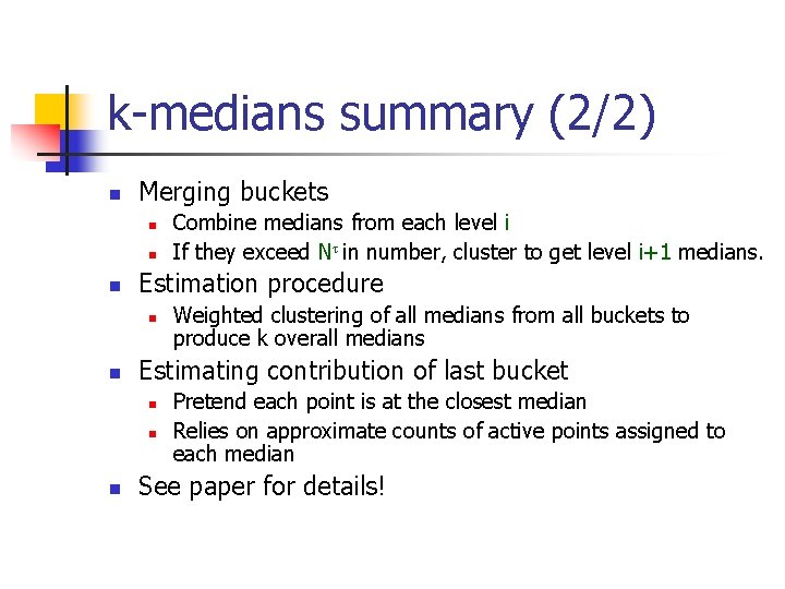
k-medians summary (2/2) n Merging buckets n n n Estimation procedure n n Weighted clustering of all medians from all buckets to produce k overall medians Estimating contribution of last bucket n n n Combine medians from each level i If they exceed Nτ in number, cluster to get level i+1 medians. Pretend each point is at the closest median Relies on approximate counts of active points assigned to each median See paper for details!

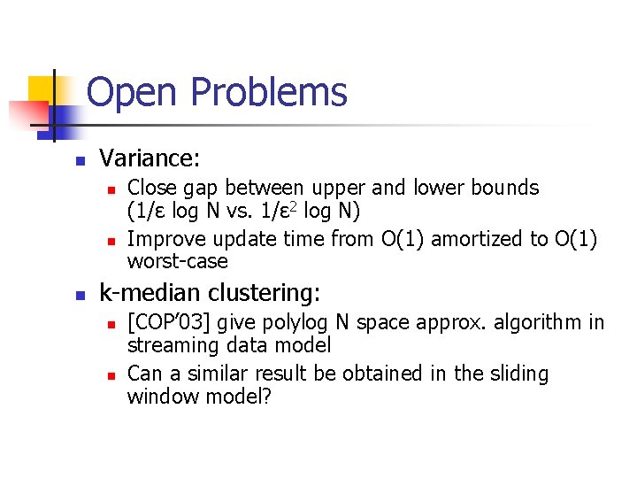
Open Problems n Variance: n n n Close gap between upper and lower bounds (1/ε log N vs. 1/ε 2 log N) Improve update time from O(1) amortized to O(1) worst-case k-median clustering: n n [COP’ 03] give polylog N space approx. algorithm in streaming data model Can a similar result be obtained in the sliding window model?

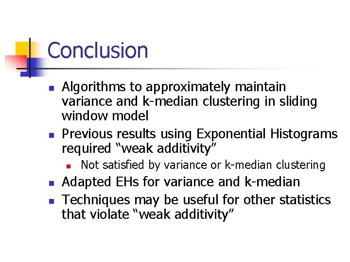
Conclusion n n Algorithms to approximately maintain variance and k-median clustering in sliding window model Previous results using Exponential Histograms required “weak additivity” n n n Not satisfied by variance or k-median clustering Adapted EHs for variance and k-median Techniques may be useful for other statistics that violate “weak additivity”