LWS Team meeting Using Direct MonteCarlo to study

LWS Team meeting Using Direct Monte-Carlo to study transport Gang Li Sep. 16 th, 2008

Motivation In using the focused transport equation to model specific event, one often assume that r or are r-independent => no radial dependence for Duu. No physical reason, probably for simplicity (easier coding for finite difference method). Direct Monte-Carlo is more intuitive, but computationally more demanding in the past. Not a problem any more. Want to explore the effect of an r-dependent Duu on particle transport --- time intensity profile, spectra, etc. Initially, has electrons in mind (injection delay between ions and electrons).

Origin of pitch angle scattering In quasi-linear theory, pitch angle scattering is caused by charged particle interacting with turbulent magnetic field. (Jokipii, 1966) The change of pitch angle is diffusive, often described by a random walk process, and the rate of change is proportional to the power of B. deterministic characteristic stochastic “scattering”–random walk

Solving the transport equation 1 a) Finite difference method (eg. Ruffolo et al 1995) 1 b) Finite difference method, add a twist of Monte-carlo in deciding . (Earl 1976, 1994) 2) Using a stochastic approach, f => f/B. Still solving f. (e. g. Qin et al. 2005) 3) Direct Monte-Carlo simulation => equations describing single particle motion. (Li et al 2008).

Fokker Planck’s coefficient D QLT limitation: slab geometry, magnetostatic. Dynamical Turbulence Bieber et al. (1994) Damping model Random sweeping model

Fokker Planck’s coefficient D (cont. ) Bieber et al. (1994) (kz - / v) (Cauchy form) (Gaussian form)

Turbulence in the solar wind Injection scales ~k-1 Injection scales Inertial range k-5/3 = energy transfer rate Inertial range Dissipation scales fc Dissipation scales Bruno et al. , 1985, q ~ -1 Leamon et al, 1999] Vasquez et al. 2007 q~ -2. 1 - -2. 5

Turbulence in the solar wind (2) Komogorov has -5/3, which is hard to distinguish from -1. 5. In different ranges, energy containing, inertial and dissipation range, q can vary a lot. consider different cases, q = 1. 5, 1. 666, 2. 5 and vary four cases. Input: 1 AU observations of the power spectrum (d. B^2) and correlation length and some r dependence of interplanetary turbulence. Output: time intensity profiles at 3 rs r = 0. 5, 1. 0, and 1. 5 AU. spectrum. anisotropy analysis [ not accomplished yet. ]

if only examine u dependence, we obtain. This, however, ignores r-dependence completely. The form of P (power spectrum), including dissipation range is: C and lambda_c in the above are the two parameters decide the power. Relate them to observed quantity through,

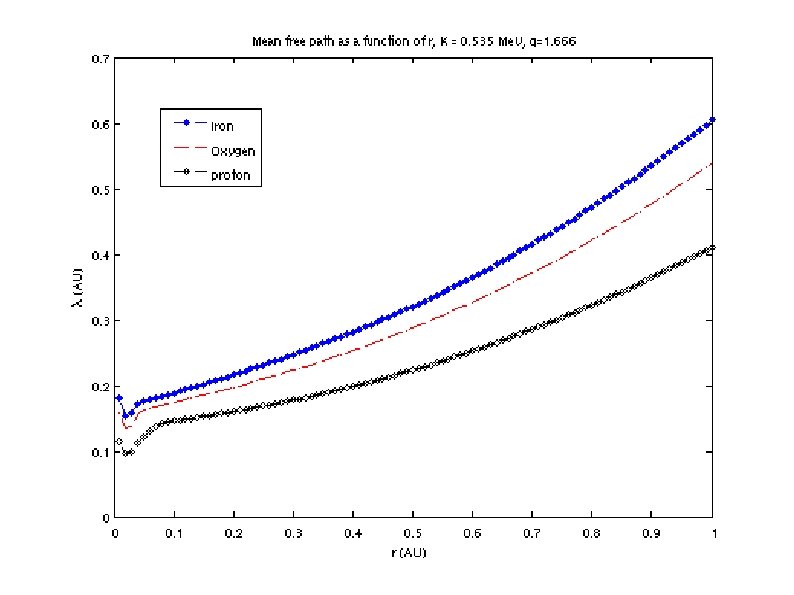
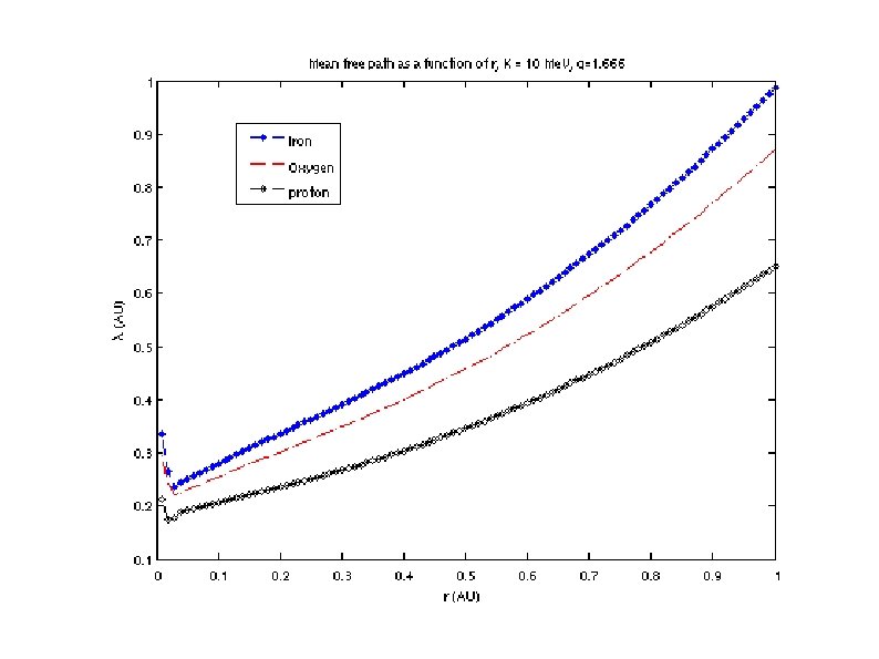
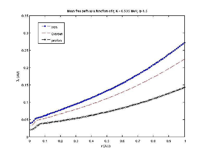
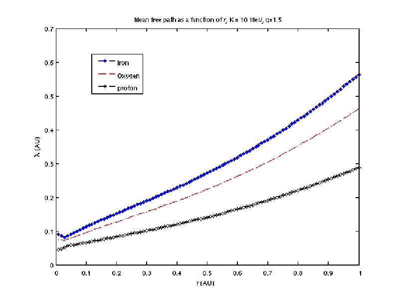
Use the same observed quantities, but different q value (since it is hard to tell the difference between 1. 5 and 1. 666) to drive the simulation. Two energies: K = 10 Me. V/nucleon and 0. 5 Me. V/nucleon, for four species: proton, Q/A = 1; Helium Q/A = 2/4, Oxygen Q/A =6/16; Iron Q/A =14/56. Simulation assumes a delta-injection in time. Plot derived quantity lambda. Plot time-intensity profiles. goal is to 1) understanding different pieces in the transort equation. 2) find similarities (resemblance) between simulation and observations ==> guidance for future work. [more realistic injection profiles, etc. ]

In this work, we keep Duu (mfp) unchanged, i. e. we use Duu with its value at (r=1 AU) throughout the simulation although previous figures show Duu change with r in a WKB approximation.

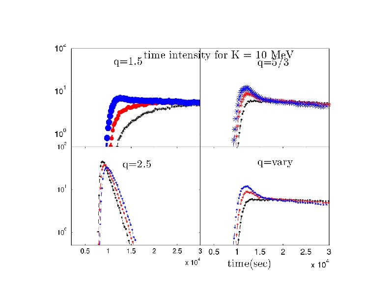
Time intensity profile at r = 1 AU

Time intensity profile at r = 1 AU

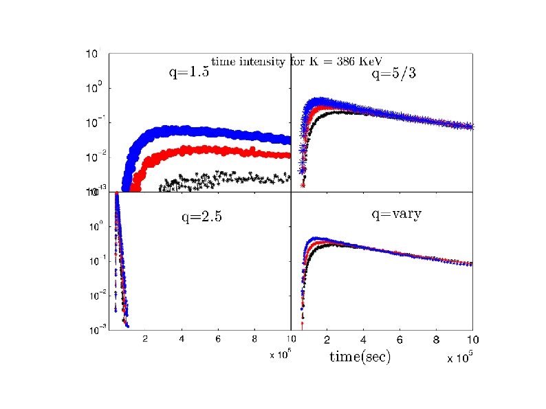
Time intensities at r = 0. 5 AU

Time intensities at r = 0. 5 AU

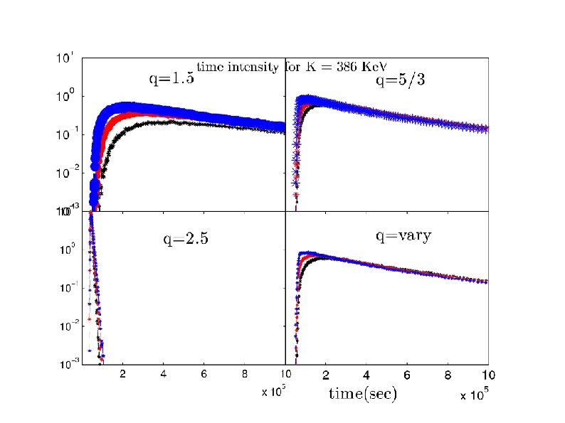
Time intensities at r = 1. 5 AU

Time intensities at r = 1. 5 AU

R-dependent Duu Blue -> proton red -> Helium blk -> iron

confident with the code. Time intensity is very sensitive to r. Helios, Solar Orbiter, Solar Probe. If Duu has no r dependence --- time intensity scales well. R-dependent Duu resembles an extended injection.