LISA Data Analysis Ron Hellings Montana State University

LISA Data Analysis Ron Hellings Montana State University - Bozeman Shane Larson California Institute of Technology with help from Matt Benacquista Montana State University - Billings

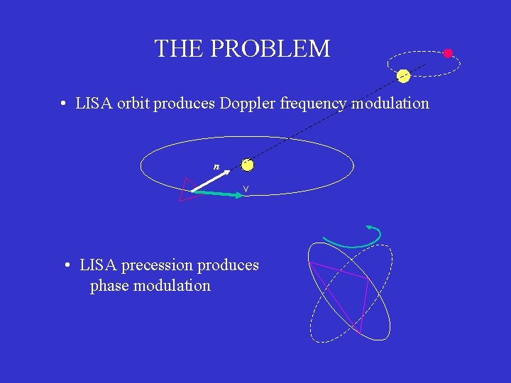
THE PROBLEM • LISA orbit produces Doppler frequency modulation n v • LISA precession produces phase modulation

hf ( 10 18) A Monochromatic Binary Signal seen in a barycentric frame f ( Hz)

hf ( 10 18) The same signal seen in an orbiting and precessing frame f ( Hz)

hf ( 10 18) The same signal seen in the presence of typical LISA noise f ( Hz)

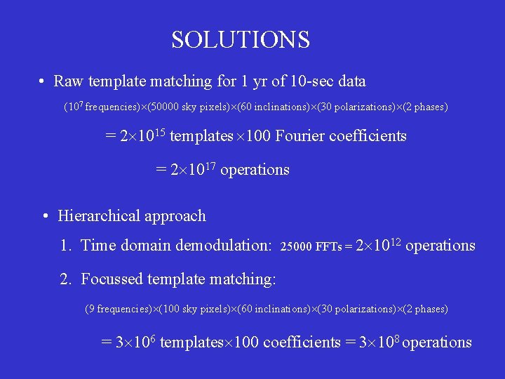
SOLUTIONS • Raw template matching for 1 yr of 10 -sec data (107 frequencies) (50000 sky pixels) (60 inclinations) (30 polarizations) (2 phases) = 2 1015 templates 100 Fourier coefficients = 2 1017 operations • Hierarchical approach 1. Time domain demodulation: 25000 FFTs = 2 1012 operations 2. Focussed template matching: (9 frequencies) (100 sky pixels) (60 inclinations) (30 polarizations) (2 phases) = 3 106 templates 100 coefficients = 3 108 operations

Let’s see how this works.

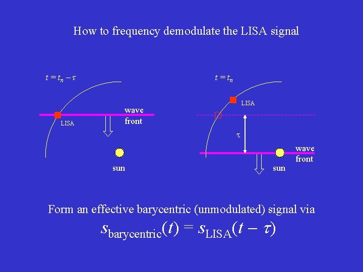
How to frequency demodulate the LISA signal t = tn LISA wave front sun wave front Form an effective barycentric (unmodulated) signal via sbarycentric(t) = s. LISA(t )

hf ( 10 18) The result of the LISA demodulation f ( Hz)

hf ( 10 18) Contrast: The same result for OMEGA f ( Hz)

Details of the Doppler demodulation • Using a simulated data file created by Matt Benacquista containing 90, 000 binary white dwarfs in the galaxy

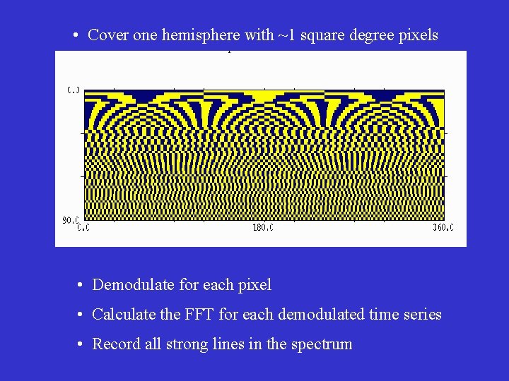
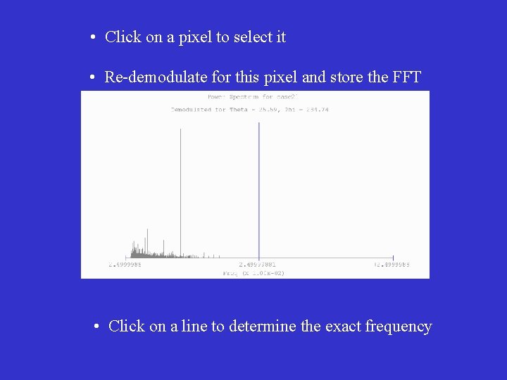
• Cover one hemisphere with ~1 square degree pixels • Demodulate for each pixel • Calculate the FFT for each demodulated time series • Record all strong lines in the spectrum

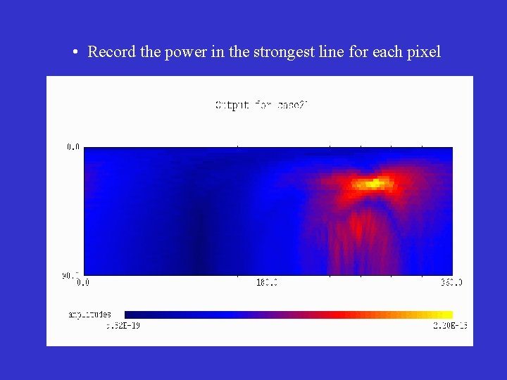
• Record the power in the strongest line for each pixel

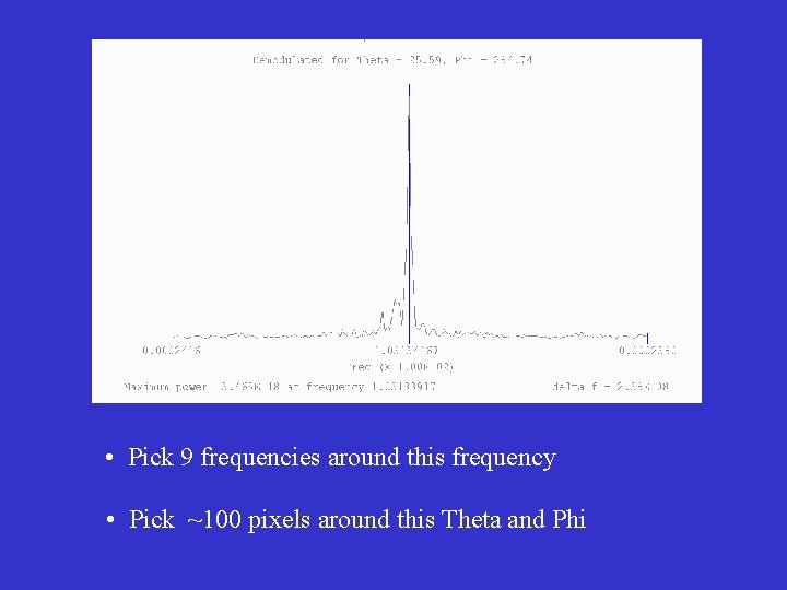
• Click on a pixel to select it • Re-demodulate for this pixel and store the FFT • Click on a line to determine the exact frequency

• Pick 9 frequencies around this frequency • Pick ~100 pixels around this Theta and Phi

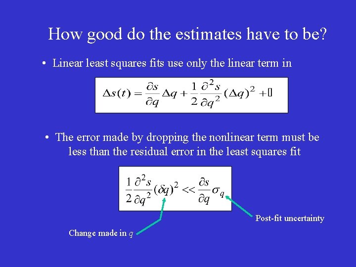
How good do the estimates have to be? • Linear least squares fits use only the linear term in • The error made by dropping the nonlinear term must be less than the residual error in the least squares fit Post-fit uncertainty Change made in q

Now what we know we can do. . . and would love to be able to show you. . . is the refined template matching using g. CLEAN. . . with only. . . 106 templates but we haven’t been able to get the damn programs to talk to each other! So to get a set of parameter values close enough to the true parameters to be in the linear regime for a least squares fit, I had to go to Matt’s file and find the parameters he used to create the time series.

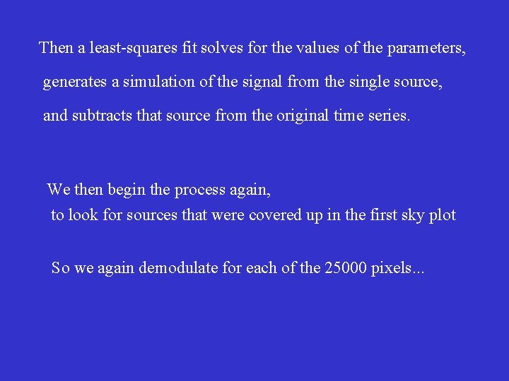
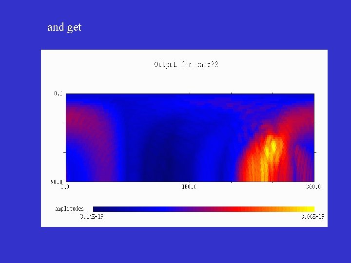
Then a least-squares fit solves for the values of the parameters, generates a simulation of the signal from the single source, and subtracts that source from the original time series. We then begin the process again, to look for sources that were covered up in the first sky plot So we again demodulate for each of the 25000 pixels. . .

and get

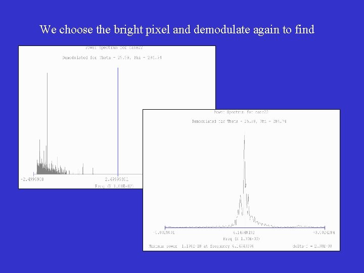
We choose the bright pixel and demodulate again to find

A Cautionary Tale

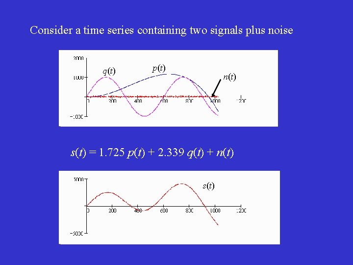
Consider a time series containing two signals plus noise q(t) p(t) n(t) s(t) = 1. 725 p(t) + 2. 339 q(t) + n(t) s(t)

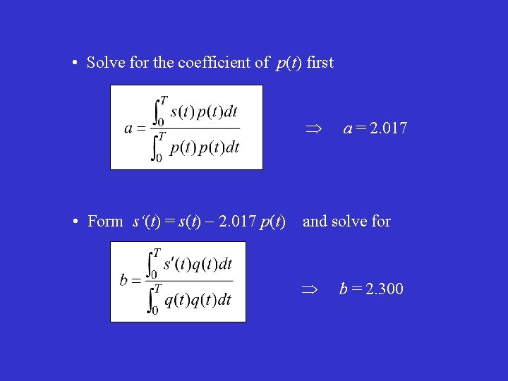
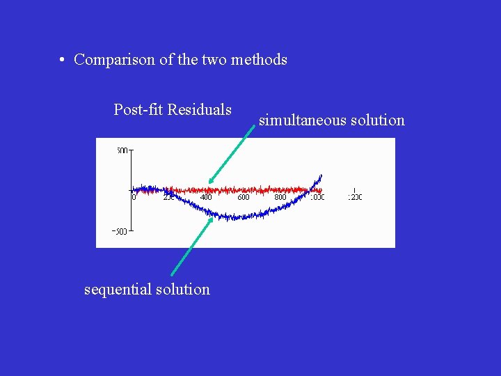
• Solve for the coefficient of p(t) first a = 2. 017 • Form s‘(t) = s(t) 2. 017 p(t) and solve for b = 2. 300

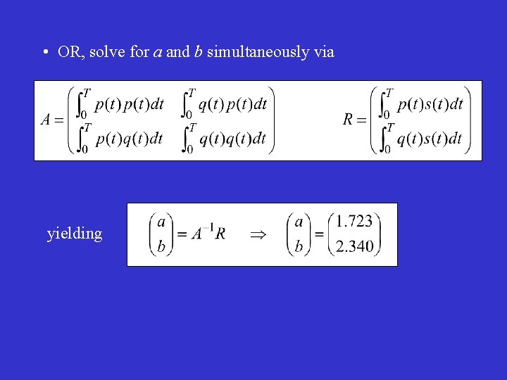
• OR, solve for a and b simultaneously via yielding

• Comparison of the two methods Post-fit Residuals sequential solution simultaneous solution

Moral: The LISA Data Analysis Method 1. 2. 3. 4. 5. 6. 7. 8. All-sky demodulate the signal Find the strongest source in the sky Form the power spectrum for its demodulation Estimate the best , , f values Refine the source parameters using templates Do a least-squares fit for ALL sources so far Form a new time series with the sources subtracted Go to 1

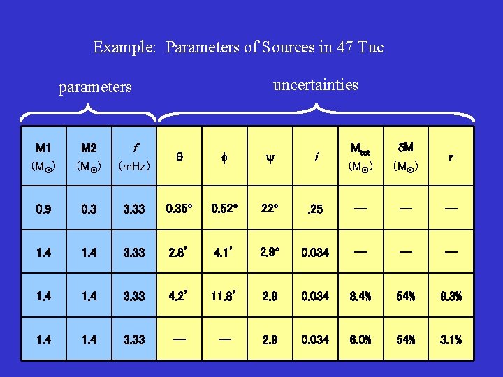
But that’s not what you came to hear. How well can this process determine parameters of binary systems in globular clusters?

Example: Parameters of Sources in 47 Tuc uncertainties parameters i Mtot (M ) M (M ) r 3. 33 0. 35 0. 52 22 . 25 -- -- -- 1. 4 3. 33 2. 8’ 4. 1’ 2. 9 0. 034 -- -- -- 1. 4 3. 33 4. 2’ 11. 8’ 2. 9 0. 034 8. 4% 54% 9. 3% 1. 4 3. 33 -- -- 2. 9 0. 034 6. 0% 54% 3. 1% f M 1 (M ) M 2 (M ) (m. Hz) 0. 9 0. 3 1. 4