Linear Models 11 Multiple Regression Models A general

Linear Models 11 ﺍﻟﻤﺤﺎﺿﺮﺓ

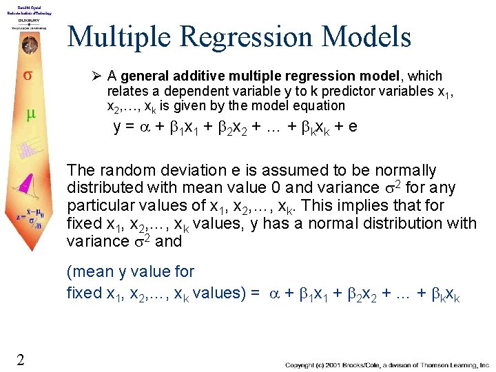
Multiple Regression Models Ø A general additive multiple regression model, which relates a dependent variable y to k predictor variables x 1, x 2, …, xk is given by the model equation y = a + b 1 x 1 + b 2 x 2 + … + bkxk + e The random deviation e is assumed to be normally distributed with mean value 0 and variance s 2 for any particular values of x 1, x 2, …, xk. This implies that for fixed x 1, x 2, …, xk values, y has a normal distribution with variance s 2 and (mean y value for fixed x 1, x 2, …, xk values) = a + b 1 x 1 + b 2 x 2 + … + bkxk 2

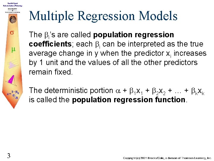
Multiple Regression Models The bi’s are called population regression coefficients; each bi can be interpreted as the true average change in y when the predictor xi increases by 1 unit and the values of all the other predictors remain fixed. The deterministic portion a + b 1 x 1 + b 2 x 2 + … + bkxk is called the population regression function. 3

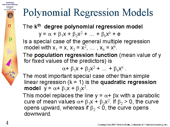
Polynomial Regression Models The kth degree polynomial regression model y = a + b 1 x + b 2 x 2 + … + bkxk + e Is a special case of the general multiple regression model with x 1 = x, x 2 = x 2, … , xk = xk. The population regression function (mean value of y for fixed values of the predictors) is a+ b 1 x + b 2 x 2 + … + bkxk. The most important special case other than simple linear regression (k = 1) is the quadratic regression model y = a+ b 1 x + b 2 x 2. This model replaces the line y = a+ bx with a parabolic cure of mean values a+ b 1 x + b 2 x 2. If b 2 > 0, the curve opens upward, whereas if b 2 < 0, the curve opens downward. 4

Interaction If the change in the mean y value associated with a 1 -unit increase in one independent variable depends on the value of a second independent variable, there is interaction between these two variables. When the variables are denoted by x 1 and x 2, such interaction can be modeled by including x 1 x 2, the product of the variables that interact, as a predictor variable. 5

Qualitative Predictor Variables. Up to now, we have only considered the inclusion of quantitative (numerical) predictor variables in a multiple regression model. Two types are very common: Ø Dichotomous variable: One with just two possible categories coded 0 and 1 Example ü Gender {male, female} ü Marriage status {married, not-married} Ø Ordinal variables: Categorical variables that have a natural ordering ü Activity level {light, moderate, heavy} coded respectively as 1, 2 and 3 ü Education level {none, elementary, secondary, college, graduate} coded respectively 1, 2, 3, 4, 5 (or for that matter any 5 consecutive integers} 6