Lecture 6 Inventory Management Chapter 11 Economic Production

Lecture 6 Inventory Management Chapter 11

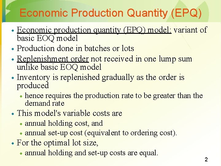
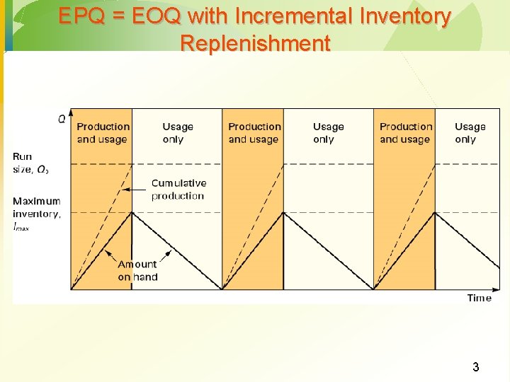
Economic Production Quantity (EPQ) · · Economic production quantity (EPQ) model: variant of basic EOQ model Production done in batches or lots Replenishment order not received in one lump sum unlike basic EOQ model Inventory is replenished gradually as the order is produced · · This model's variable costs are · · · hence requires the production rate to be greater than the demand rate annual holding cost, and annual set-up cost (equivalent to ordering cost). For the optimal lot size, · annual holding and set-up costs are equal. 2

EPQ = EOQ with Incremental Inventory Replenishment 3

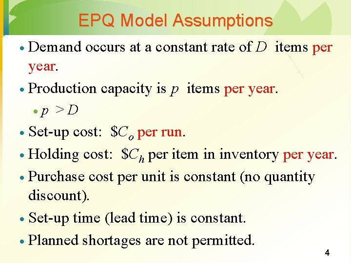
EPQ Model Assumptions Demand occurs at a constant rate of D items per year. · Production capacity is p items per year. · · p >D Set-up cost: $Co per run. · Holding cost: $Ch per item in inventory per year. · Purchase cost per unit is constant (no quantity discount). · Set-up time (lead time) is constant. · Planned shortages are not permitted. · 4

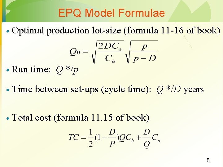
EPQ Model Formulae · Optimal production lot-size (formula 11 -16 of book) · Run time: Q */p · Time between set-ups (cycle time): Q */D years · Total cost (formula 11. 15 of book) 5

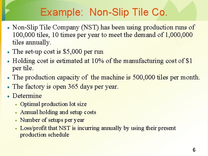
Example: Non-Slip Tile Co. · · · Non-Slip Tile Company (NST) has been using production runs of 100, 000 tiles, 10 times per year to meet the demand of 1, 000 tiles annually. The set-up cost is $5, 000 per run Holding cost is estimated at 10% of the manufacturing cost of $1 per tile. The production capacity of the machine is 500, 000 tiles per month. The factory is open 365 days per year. Determine · · Optimal production lot size Annual holding and setup costs Number of setups per year Loss/profit that NST is incurring annually by using their present production schedule 6

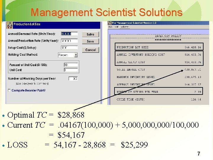
Management Scientist Solutions · · · Optimal TC = $28, 868 Current TC =. 04167(100, 000) + 5, 000, 000/100, 000 = $54, 167 LOSS = 54, 167 - 28, 868 = $25, 299 7

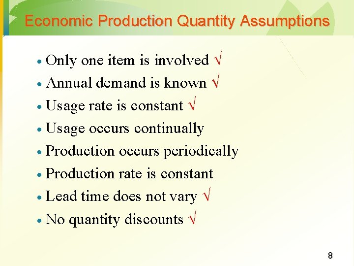
Economic Production Quantity Assumptions Only one item is involved · Annual demand is known · Usage rate is constant · Usage occurs continually · Production occurs periodically · Production rate is constant · Lead time does not vary · No quantity discounts · 8

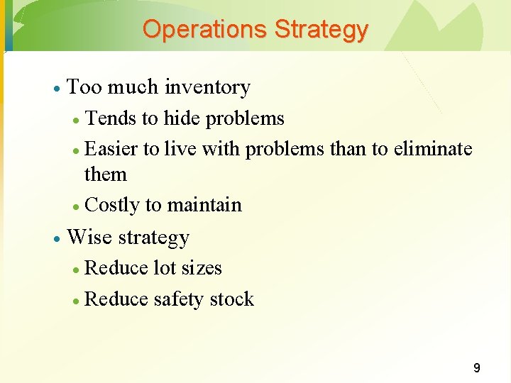
Operations Strategy · Too much inventory Tends to hide problems · Easier to live with problems than to eliminate them · Costly to maintain · · Wise strategy Reduce lot sizes · Reduce safety stock · 9

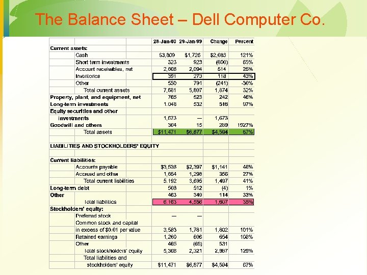
The Balance Sheet – Dell Computer Co.

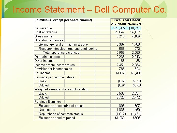
Income Statement – Dell Computer Co. (in millions, except per share amount) Net revenue Cost of revenue Gross margin Operating expenses: Selling, general and administrative Research, development, and engineering Total operating expenses Operating income Other income Income before income taxes Provision for income taxes Net income Earnings per common share: Basic Diluted Weighted average shares outstanding: Basic Diluted Retained Earnings: Balances at beginning of period Net income Repurchase of common stocks Balances at end of period Fiscal Year Ended 28 -Jan-00 29 -Jan-99 $25, 265 $18, 243 20, 047 14, 137 5, 218 4, 106 2, 387 568 2, 955 2, 263 188 2, 451 785 $1, 666 1, 788 272 2, 060 2, 046 38 2, 084 624 $1, 460 $0. 66 $0. 61 $0. 58 $0. 53 2, 536 2, 728 2, 531 2, 772 606 1, 666 (1, 012) $1, 260 607 1, 460 (1, 461) $606

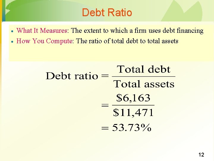
Debt Ratio · · What It Measures: The extent to which a firm uses debt financing How You Compute: The ratio of total debt to total assets 12

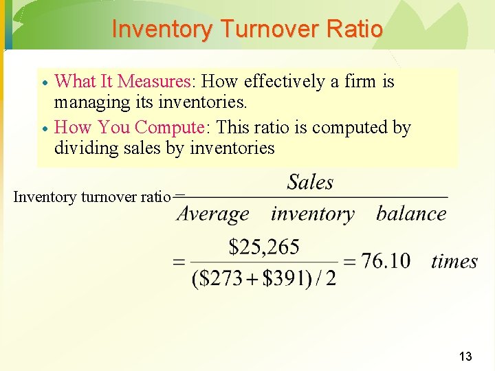
Inventory Turnover Ratio · · What It Measures: How effectively a firm is managing its inventories. How You Compute: This ratio is computed by dividing sales by inventories Inventory turnover ratio = 13

Lecture 6 MGMT 650 Simulation – Chapter 13

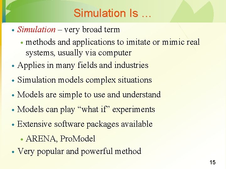
Simulation Is … · Simulation – very broad term · methods and applications to imitate or mimic real systems, usually via computer Applies in many fields and industries · Simulation models complex situations · Models are simple to use and understand · Models can play “what if” experiments · Extensive software packages available · ARENA, Pro. Model Very popular and powerful method · · 15

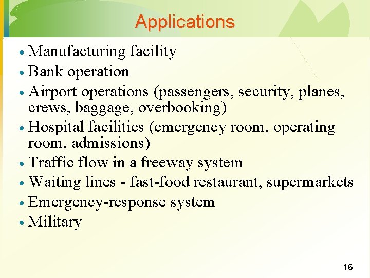
Applications Manufacturing facility · Bank operation · Airport operations (passengers, security, planes, crews, baggage, overbooking) · Hospital facilities (emergency room, operating room, admissions) · Traffic flow in a freeway system · Waiting lines - fast-food restaurant, supermarkets · Emergency-response system · Military · 16

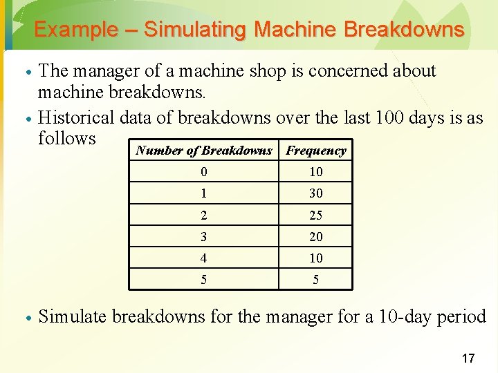
Example – Simulating Machine Breakdowns · · The manager of a machine shop is concerned about machine breakdowns. Historical data of breakdowns over the last 100 days is as follows Number of Breakdowns Frequency · 0 10 1 30 2 25 3 20 4 10 5 5 Simulate breakdowns for the manager for a 10 -day period 17

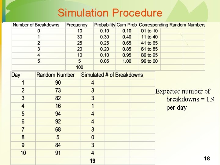
Simulation Procedure Expected number of breakdowns = 1. 9 per day 18

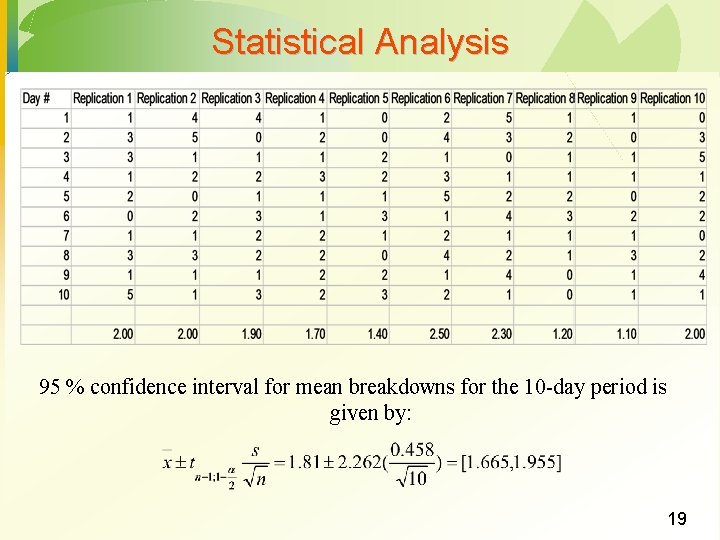
Statistical Analysis 95 % confidence interval for mean breakdowns for the 10 -day period is given by: 19

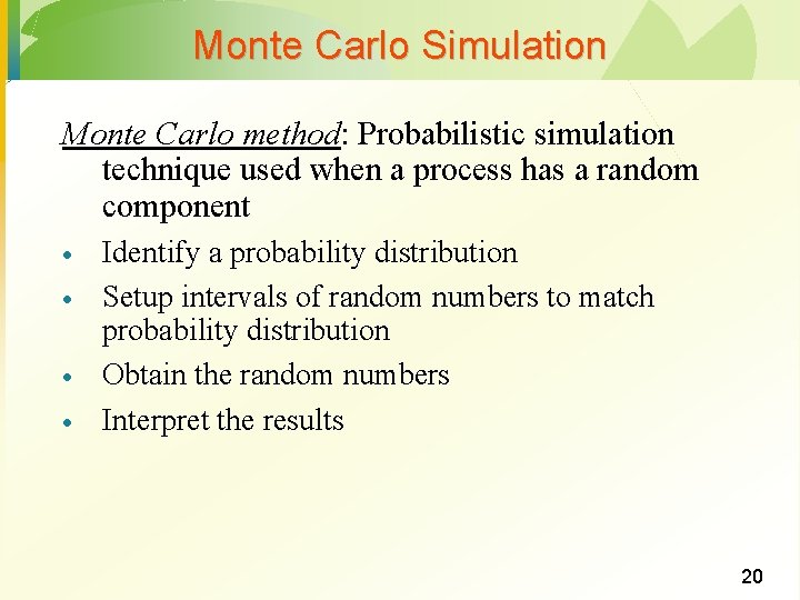
Monte Carlo Simulation Monte Carlo method: Probabilistic simulation technique used when a process has a random component · · Identify a probability distribution Setup intervals of random numbers to match probability distribution Obtain the random numbers Interpret the results 20

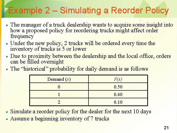
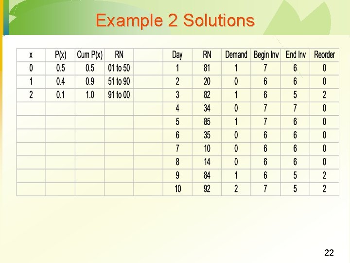
Example 2 – Simulating a Reorder Policy · · · The manager of a truck dealership wants to acquire some insight into how a proposed policy for reordering trucks might affect order frequency Under the new policy, 2 trucks will be ordered every time the inventory of trucks is 5 or lower Due to proximity between the dealership and the local office, orders can be filled overnight The “historical” probability for daily demand is as follows Demand (x) P(x) 0 0. 50 1 0. 40 2 0. 10 Simulate a reorder policy for the dealer for the next 10 days Assume a beginning inventory of 7 trucks 21

Example 2 Solutions 22

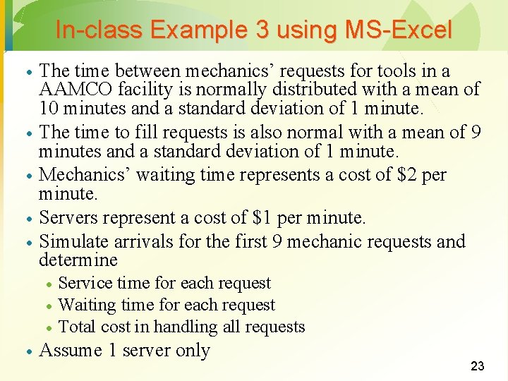
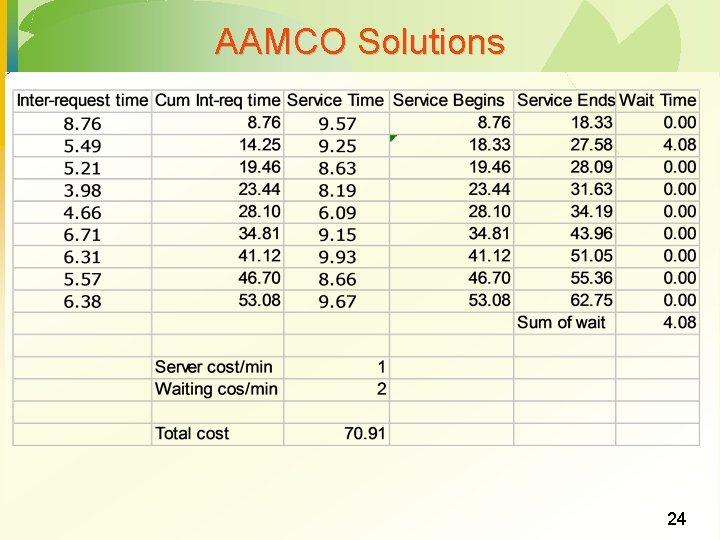
In-class Example 3 using MS-Excel · · · The time between mechanics’ requests for tools in a AAMCO facility is normally distributed with a mean of 10 minutes and a standard deviation of 1 minute. The time to fill requests is also normal with a mean of 9 minutes and a standard deviation of 1 minute. Mechanics’ waiting time represents a cost of $2 per minute. Servers represent a cost of $1 per minute. Simulate arrivals for the first 9 mechanic requests and determine · · Service time for each request Waiting time for each request Total cost in handling all requests Assume 1 server only 23

AAMCO Solutions 24

Simulation Models Are Beneficial Systematic approach to problem solving · Increase understanding of the problem · Enable “what if” questions · Specific objectives · Power of mathematics and statistics · Standardized format · Require users to organize · 25

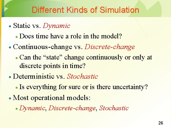
Different Kinds of Simulation · Static vs. Dynamic · · Continuous-change vs. Discrete-change · · Can the “state” change continuously or only at discrete points in time? Deterministic vs. Stochastic · · Does time have a role in the model? Is everything for sure or is there uncertainty? Most operational models: · Dynamic, Discrete-change, Stochastic 26

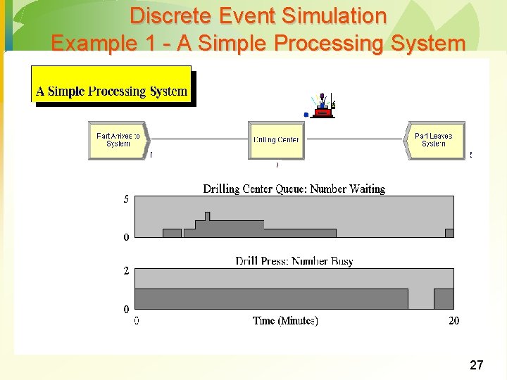
Discrete Event Simulation Example 1 - A Simple Processing System 27

Advantages of Simulation Solves problems that are difficult or impossible to solve mathematically · Flexibility to model things as they are (even if messy and complicated) · Allows experimentation without risk to actual system · · Ability to model long-term effects · Serves as training tool for decision makers 28

Limitations of Simulation · Does not produce optimum solution · Model development may be difficult · Computer run time may be substantial · Monte Carlo simulation only applicable to random systems 29

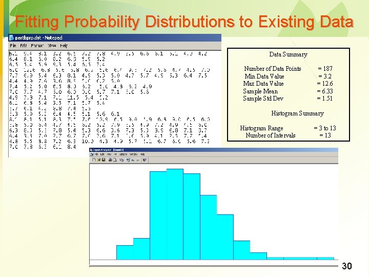
Fitting Probability Distributions to Existing Data Summary Number of Data Points Min Data Value Max Data Value Sample Mean Sample Std Dev = 187 = 3. 2 = 12. 6 = 6. 33 = 1. 51 Histogram Summary Histogram Range Number of Intervals = 3 to 13 = 13 30

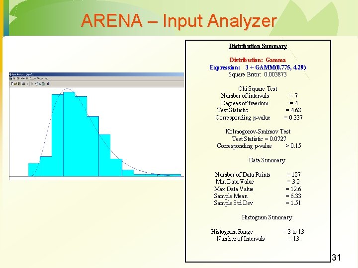
ARENA – Input Analyzer Distribution Summary Distribution: Gamma Expression: 3 + GAMM(0. 775, 4. 29) Square Error: 0. 003873 Chi Square Test Number of intervals Degrees of freedom Test Statistic Corresponding p-value =7 =4 = 4. 68 = 0. 337 Kolmogorov-Smirnov Test Statistic = 0. 0727 Corresponding p-value > 0. 15 Data Summary Number of Data Points Min Data Value Max Data Value Sample Mean Sample Std Dev = 187 = 3. 2 = 12. 6 = 6. 33 = 1. 51 Histogram Summary Histogram Range Number of Intervals = 3 to 13 = 13 31

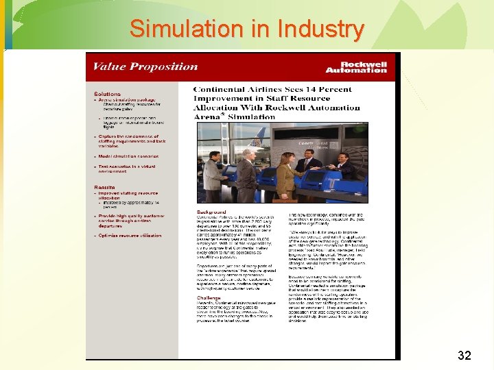
Simulation in Industry 32

Course Conclusions · · Recognize that not every tool is the best fit for every problem Pay attention to variability · Forecasting · Inventory management - Deliveries from suppliers Build flexibility into models Pay careful attention to technology · Opportunities · · Improvement in service and response times Risks · Costs involved · Difficult to integrate · Need for periodic updates · Requires training · Garbage in, garbage out · Results and recommendations you present are only as reliable as the model and its inputs · Most decisions involve tradeoffs Not a good idea to make decisions to the exclusion of known information · 33