Lecture 16 Time Series and Stochastic Processes Thursday

Lecture 16 Time Series and Stochastic Processes Thursday, October 21, 1999 William H. Hsu Department of Computing and Information Sciences, KSU http: //www. cis. ksu. edu/~bhsu Readings: Chapter 16, Russell and Norvig “The Future of Time Series: Learning and Understanding”, Gershenfeld and Weigend CIS 798: Intelligent Systems and Machine Learning Kansas State University Department of Computing and Information Sciences

Lecture Outline • Readings: Chapter 16, Russell and Norvig • Exercise: 16. 1(a), Russell and Norvig (Bring Answers to Class) • Introduction to Time Series – Time series analysis • Forecasting (prediction) • Modeling • Characterization – Probability and time series: stochastic processes – Representations: linear models – Time series understanding and learning • Understanding: state-space reconstruction • Learning: parameter estimation (e. g. , using artificial neural networks) • Next Lecture: Policy Learning, Markov Decision Processes (MDPs) – Read Chapter 17, Russell and Norvig – Read Sections 13. 1 -13. 2, Mitchell CIS 798: Intelligent Systems and Machine Learning Kansas State University Department of Computing and Information Sciences

Time Series Analysis • Problems – Given: observations of a system through time (historical data D) – Forecasting, aka prediction: predict the short-term behavior of system – Modeling: find a description for the long-term behavior of system – Characterization: determine fundamental properties of system with no prior knowledge • Forecasting – Simple (“traditional”): extrapolation (windowing, smoothing) methods – “Modern”: linear models - e. g. , weighted sum of previous observations + noise • Modeling – Fitting model components to capture system behavior (read: finding hypothesis) – Parameter estimation: maximizing P( | D) • Characterization – Example: determining number of degrees of freedom; clusters; randomness – Model selection: sometimes uses such characterization CIS 798: Intelligent Systems and Machine Learning Kansas State University Department of Computing and Information Sciences

Forecasting • Framework – Given: observations D {x(t 0), x(t 1), …, x(tm)} where x(ti) (x 1(ti), x 2(ti), …, xn(ti)) – Predict: a continuation of {x(t)}, e. g. , x(tm+1), x(tm+2), …, x(tm+k) for “small” k – Forecasting : time series analysis : : performance element : learning system • Decision Support Applications – Prognostic monitoring: crises, resource demand, business simulations – Recommender systems: precision agriculture, patent intelligence, logistics – Control automation: damage control, manufacturing, negotiation, web agents • Solution Approaches – Predict with linear model: compute estimated function of previous observations – Bayesian methods: integrate predictions over a hypothesis space H • Role of Learning – Characterizing {x(t)} to choose a hypothesis language (e. g. , type of linear model) – Modeling: acquiring predictive model of {x(t)} – Forecasting: applying predictive model CIS 798: Intelligent Systems and Machine Learning Kansas State University Department of Computing and Information Sciences

Learning to Forecast (Predict) Time Series • Old Solution: Pure Extrapolation – Pure extrapolation: fit a curve through all the points (in time domain) – Use to generate predictions: plug in tm+k as dependent variable • Problems with Old Solution – Doesn’t capture local dependencies (e. g. , periodicities) – Very sensitive to noise; cannot adequately isolate it • New Solutions – Linear models: estimate function over past observations • e. g. , fixed “window”; decaying average of all past observations; both • Use estimate (hypothesis) to generate points of the continuation • Problems with this approach: typically can’t prove system behaves this way – Characterization: understanding the pattern-generating process • Time-delay embedding: change of representation for dynamical system • State-space reconstruction: finding hypotheses in transformed space – Modeling: using this knowledge to guide learning (parameter estimation) CIS 798: Intelligent Systems and Machine Learning Kansas State University Department of Computing and Information Sciences

Modeling • Framework – Given: D {x(t 0), x(t 1), …, x(tm)} – Return: a hypothesis h H such that h(D) predicts {x(tm+1), x(tm+2), …, x(tm+k)} – Compare: classifier learning (return h, use to classify: h(x) = c(x), h(x) = v(x)) • Issues – May need to transform X to X’: e. g. , time domain frequency domain – Just as with classification, probabilistic methods may estimate v. MAP or v. BOC • Solution Approaches – Train artificial neural network (ANN) to map from {x(ti-k), x(ti-k+1), …, x(ti)} to x(ti+1) • Can a static (i. e. , atemporal) feedforward ANN express the relationship? • Can perform change of representation (embedding) using recurrent ANN – Other classifiers: e. g. , Hidden Markov Model (HMM), IBL (e. g. , k-d trees), etc. • Role of Learning – Works in conjunction with characterization (meta-learning) step – Modeling: the core learning step – Performance element: apply (query) to generate predictions, responses CIS 798: Intelligent Systems and Machine Learning Kansas State University Department of Computing and Information Sciences

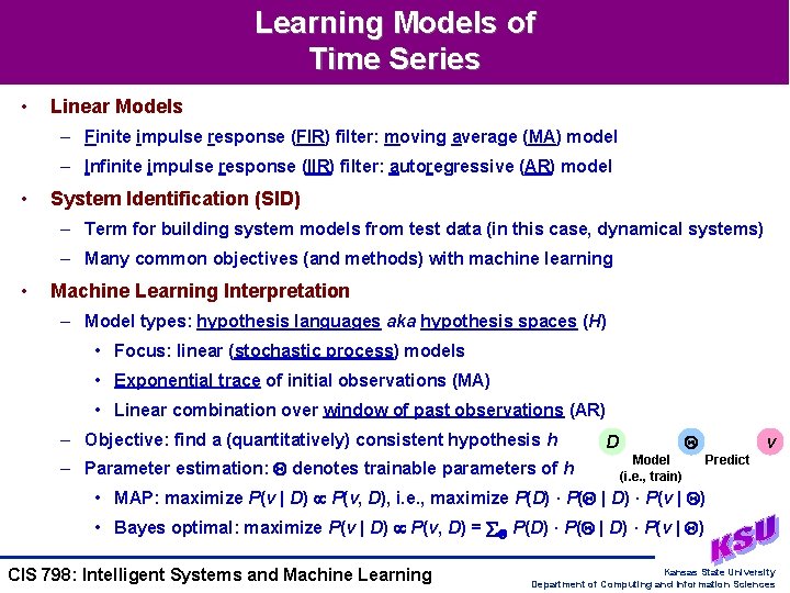
Learning Models of Time Series • Linear Models – Finite impulse response (FIR) filter: moving average (MA) model – Infinite impulse response (IIR) filter: autoregressive (AR) model • System Identification (SID) – Term for building system models from test data (in this case, dynamical systems) – Many common objectives (and methods) with machine learning • Machine Learning Interpretation – Model types: hypothesis languages aka hypothesis spaces (H) • Focus: linear (stochastic process) models • Exponential trace of initial observations (MA) • Linear combination over window of past observations (AR) – Objective: find a (quantitatively) consistent hypothesis h – Parameter estimation: denotes trainable parameters of h D Model (i. e. , train) v Predict • MAP: maximize P(v | D) P(v, D), i. e. , maximize P(D) · P( | D) · P(v | ) • Bayes optimal: maximize P(v | D) P(v, D) = P(D) · P( | D) · P(v | ) CIS 798: Intelligent Systems and Machine Learning Kansas State University Department of Computing and Information Sciences

Characterization • Framework – Given: observations D – Develop: description of H • Characterization: use this description to select parameters • Modeling: use this description to select parameter values • Direct versus Indirect Characterization – Direct: find transformation of X, H into better-understood X’, H’ – Indirect: train models, study h’s to describe H (“understanding through learning”) • Solution Approaches – Model selection: searching H using probabilistic criteria (e. g. , MDL / BIC) – Direct characterization: state-space reconstruction (by delay-space embedding) – Indirect: post-visualizations of ANN performance; statistical validation; etc. • Role of Learning – Characterization: the meta-learning step – Apply to control learning (modeling) step and produce predictions – NB: may need to implement using clustering (to transform X), wrapper CIS 798: Intelligent Systems and Machine Learning Kansas State University Department of Computing and Information Sciences

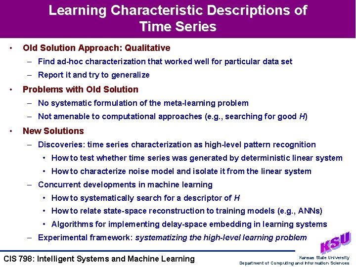
Learning Characteristic Descriptions of Time Series • Old Solution Approach: Qualitative – Find ad-hoc characterization that worked well for particular data set – Report it and try to generalize • Problems with Old Solution – No systematic formulation of the meta-learning problem – Not amenable to computational approaches (e. g. , searching for good H) • New Solutions – Discoveries: time series characterization as high-level pattern recognition • How to test whether time series was generated by deterministic linear system • How to characterize noise model and isolate it from the linear system – Concurrent developments in machine learning • How to systematically search for a descriptor of H • How to relate state-space reconstruction to training models (e. g. , ANNs) • Algorithms for implementing delay-space embedding in learning systems – Experimental framework: systematizing the high-level learning problem CIS 798: Intelligent Systems and Machine Learning Kansas State University Department of Computing and Information Sciences

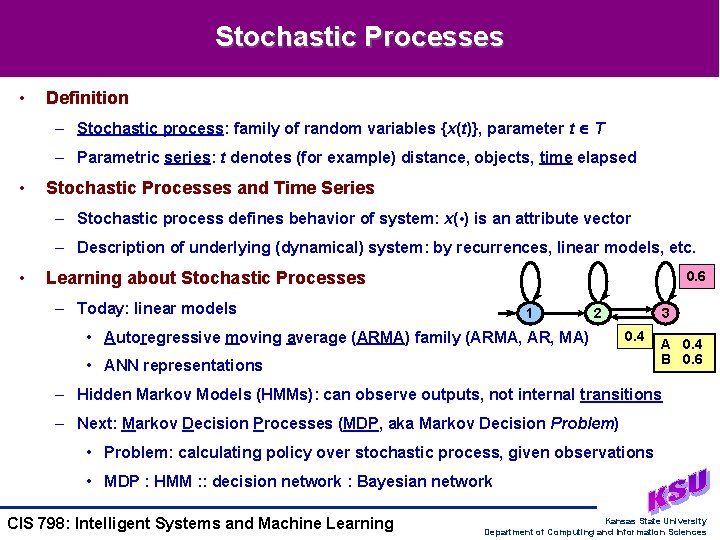
Stochastic Processes • Definition – Stochastic process: family of random variables {x(t)}, parameter t T – Parametric series: t denotes (for example) distance, objects, time elapsed • Stochastic Processes and Time Series – Stochastic process defines behavior of system: x( • ) is an attribute vector – Description of underlying (dynamical) system: by recurrences, linear models, etc. • Learning about Stochastic Processes 0. 6 – Today: linear models 1 2 • Autoregressive moving average (ARMA) family (ARMA, AR, MA) 3 0. 4 • ANN representations A 0. 4 B 0. 6 – Hidden Markov Models (HMMs): can observe outputs, not internal transitions – Next: Markov Decision Processes (MDP, aka Markov Decision Problem) • Problem: calculating policy over stochastic process, given observations • MDP : HMM : : decision network : Bayesian network CIS 798: Intelligent Systems and Machine Learning Kansas State University Department of Computing and Information Sciences

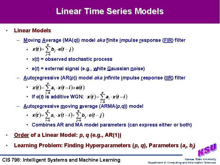
Linear Time Series Models • Linear Models – Moving Average (MA(q)) model aka finite impulse response (FIR) filter • • x(t) = observed stochastic process • e(t) = external signal (e. g. , white Gaussian noise) – Autoregressive (AR(p)) model aka infinite impulse response (IIR) filter • • If e(t) is additive WGN: – Autoregressive moving average (ARMA(p, q)) model • • Combines AR and MA model parameters (can express either or both) • Order of a Linear Model: p, q (e. g. , AR(1)) • Learning Problem: Finding Hyperparameters (p, q), Parameters (ai, bj) CIS 798: Intelligent Systems and Machine Learning Kansas State University Department of Computing and Information Sciences

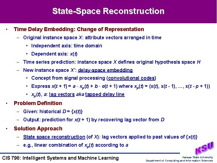
State-Space Reconstruction • Time Delay Embedding: Change of Representation – Original instance space X: attribute vectors arranged in time • Independent axis: time domain • Dependent axis: x(t) – Time series prediction: instance space X defines original hypothesis space H – New instance space X’: delay-space embedding • Concept from signal processing (convolutional codes) • Express x(t + 1) = a · xp(t) + b · e(t + 1) where xp(t) = (x(t), x(t - 1), …, x(t - p + 1)) • xp(t), a: lag vectors aka tapped delay line • Problem Definition – Given: historical D = {x(t)} – Output: prediction for x(t + 1) by recovering lag vector from D • Solution Approach – State space reconstruction (of X): lag vectors applied to past values of {x(t)} – e. g. , linear combination of xp(t) according to a CIS 798: Intelligent Systems and Machine Learning Kansas State University Department of Computing and Information Sciences

Neural Networks for Time Series Learning • Problem: Acquire Linear Model (Estimate Parameters) • Solution Approach – Models • Simple recurrent networks (SRNs) [Jordan, 1987; Elman, 1990] • Time-delay neural networks (TDNNs, aka tapped delay line neural networks) [Lang, Waibel, and Hinton, 1990] • Gamma memories: [Principe and de. Vries, 1992] – Learning algorithms for temporal ANNs • Backpropagation through time (BPTT) [Rumelhart et al, 1986] • Real-time recurrent learning (RTRL) [Williams and Zipser, 1989] • Subtypes of Simple Recurrent Networks (SRNs) – Input recurrent (IR): input-to-input unit feedback; exponential trace (~MA(1)) – Elman: hidden-to-input unit feedback; no linear model characterization known – Jordan: output-to-input unit feedback; autoregressive (~AR) CIS 798: Intelligent Systems and Machine Learning Kansas State University Department of Computing and Information Sciences

Connectionist Time Series Learning: ARMA Characterization • Implementing Delay-Space Embedding – Lag vector xp(t) can be captured by TDNN – Gamma memory: a low-order ARMA model • Depth versus Resolution – Depth: non-Markovity, i. e. , P(x(t + 1) | xp(t)) P(x(t + 1) | x(t)) – Resolution: representation accuracy at a particular lag (delay) value – TDNNs: high resolution, low depth; IR networks: low resolution, high depth – Gamma memories: high resolution, high depth (and high complexity!) • Forecasting with Temporal ANNs – References • Mozer, 1994; Mehrotra, Mohan, and Ranka, 1997: kernel functions • Haykin, 1994; Hassoun, 1995: BPTT, RTRL • Bishop, 1995: one-step ahead versus multi-step ahead prediction • Hsu, 1998: mixtures of temporal ANNs (SRNs, TDNNs, Gamma memories) – Issue: generating continuations - how useful is it to look further ahead? CIS 798: Intelligent Systems and Machine Learning Kansas State University Department of Computing and Information Sciences

Santa Fe Institute Time Series Learning Competition • Competition – One of first open computing challenges on Internet (1991) – “Only” several megabytes of data (FTP, floppy distribution) – Ran from 8/1/1991 - 1/15/1992; results in book (Gershenfeld and Weigend, 1994) – Objective: to provide benchmark corpus and representative test standard • Web Site: http: //www. stern. nyu. edu/~aweigend/Time-Series/Santa. Fe. html – Several data sets from competition in online archive, for you to try – Research benchmark for time series learning models, algorithms, approaches • Six Data Sets – Laser intensity level (far-infrared) – Sleep apnea patient readings (heart rate, chest volume, blood O 2, EEG rate) – High-frequency currency exchange rate (Swiss franc versus U. S. dollar) – Synthetic dynamical system – Astrophysical data (intensity of white dwarf star; noisy measurements) – J. S. Bach’s last, unfinished fugue from The Art of the Fugue CIS 798: Intelligent Systems and Machine Learning Kansas State University Department of Computing and Information Sciences

Time Series and Policy Learning • Problem Definition – Given • Stochastic environment: outcome P(Result (action) | Do(action), state) • State: totally observable (accessible) or partially observable (inaccessible) – Return: a policy f : state action • Foundations of Policy Learning – Utilities: U: state value – Markov Decision Processes: next • Solution Approaches – Value iteration: utility decomposes according to reward function • Calculate utilities of each state • Use state utilities to select optimal action a, given inferred state – Policy iteration: utility decomposes according reward function, policies • Pick a policy; calculate utilities of each state given the policy • Modify policy to include optimal action, given inferred state CIS 798: Intelligent Systems and Machine Learning Kansas State University Department of Computing and Information Sciences

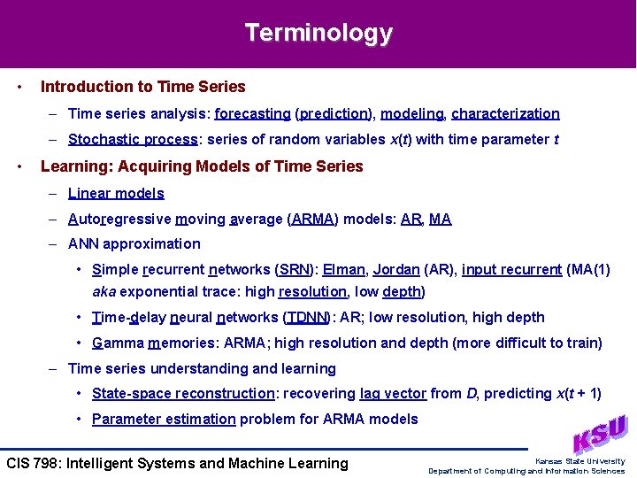
Terminology • Introduction to Time Series – Time series analysis: forecasting (prediction), modeling, characterization – Stochastic process: series of random variables x(t) with time parameter t • Learning: Acquiring Models of Time Series – Linear models – Autoregressive moving average (ARMA) models: AR, MA – ANN approximation • Simple recurrent networks (SRN): Elman, Jordan (AR), input recurrent (MA(1) aka exponential trace: high resolution, low depth) • Time-delay neural networks (TDNN): AR; low resolution, high depth • Gamma memories: ARMA; high resolution and depth (more difficult to train) – Time series understanding and learning • State-space reconstruction: recovering lag vector from D, predicting x(t + 1) • Parameter estimation problem for ARMA models CIS 798: Intelligent Systems and Machine Learning Kansas State University Department of Computing and Information Sciences

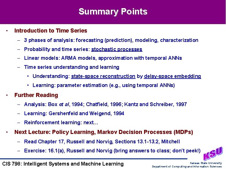
Summary Points • Introduction to Time Series – 3 phases of analysis: forecasting (prediction), modeling, characterization – Probability and time series: stochastic processes – Linear models: ARMA models, approximation with temporal ANNs – Time series understanding and learning • Understanding: state-space reconstruction by delay-space embedding • Learning: parameter estimation (e. g. , using temporal ANNs) • Further Reading – Analysis: Box et al, 1994; Chatfield, 1996; Kantz and Schreiber, 1997 – Learning: Gershenfeld and Weigend, 1994 – Reinforcement learning: next… • Next Lecture: Policy Learning, Markov Decision Processes (MDPs) – Read Chapter 17, Russell and Norvig, Sections 13. 1 -13. 2, Mitchell – Exercise: 16. 1(a), Russell and Norvig (bring answers to class; don’t peek!) CIS 798: Intelligent Systems and Machine Learning Kansas State University Department of Computing and Information Sciences