Lecture 11 Multicollinearity BMTRY 701 Biostatistical Methods II

Multicollinearity Introduction § Some common questions we ask in MLR • what is the relative importance of the effects of the different covariates? • what is the magnitude of effect of a given covariate on the response? • can any covariate be dropped from the model because it has little effect or no effect on the outcome? • should any covariates not yet included in the model be considered for possible inclusion?

Easy answers? § If the candidate covariates are uncorrelated with one another: yes, these are simple questions § If the candidate covariates are correlated with one another: no, these are not easy. § Most commonly: • observational studies have correlated covariates • we need to adjust for these when assessing relationships • “adjusting” for confounders § Experimental designs? • less problematic • patients are randomized in common designs • no confounding exists because factors are ‘balanced’ across arms

Multicollinearity § Also called “intercorrelation” § refers to the situation when the covariates are related to each other and to the outcome of interest § like confounding, but a statistical terminology for it because of the effects it has on regression modeling

No Multicollinearity Example: Mouse experiment Mouse Dose A Dose B Diet Tumor size 1 100 25 0 45 2 200 25 0 56 3 300 25 4 100 50 0 15 5 200 50 0 17 6 300 50 0 10 7 100 25 1 30 8 200 25 1 28 9 300 25 1 20 10 100 50 1 10 11 200 50 1 5 12 300 50 1 3

Linear modeling § Interested in seeing which factors influence tumor size in mice § Notice that the experiment is perfectly balanced. § What does that mean?

Dose of Drug A on Tumor > reg. a <- lm(Tumor. size ~ Dose. A, data=data) > summary(reg. a) Coefficients: Estimate Std. Error t value Pr(>|t|) (Intercept) 32. 50000 12. 29041 2. 644 0. 0246 * Dose. A -0. 05250 0. 05689 -0. 923 0. 3779 --Signif. codes: 0 ‘***’ 0. 001 ‘**’ 0. 01 ‘*’ 0. 05 ‘. ’ 0. 1 ‘ ’ 1 Residual standard error: 16. 09 on 10 degrees of freedom Multiple R-Squared: 0. 07847, Adjusted R-squared: -0. 01368 F-statistic: 0. 8515 on 1 and 10 DF, p-value: 0. 3779 >

Dose of Drug B on Tumor > reg. b <- lm(Tumor. size ~ Dose. B, data=data) > summary(reg. b) Coefficients: Estimate Std. Error t value (Intercept) 58. 0000 9. 4956 6. 108 Dose. B -0. 9600 0. 2402 -3. 996 --Signif. codes: 0 ‘***’ 0. 001 ‘**’ 0. 01 Pr(>|t|) 0. 000114 *** 0. 002533 ** ‘*’ 0. 05 ‘. ’ 0. 1 ‘ ’ 1 Residual standard error: 10. 4 on 10 degrees of freedom Multiple R-Squared: 0. 6149, Adjusted R-squared: 0. 5764 F-statistic: 15. 97 on 1 and 10 DF, p-value: 0. 002533 >

Diet on Tumor > reg. diet <- lm(Tumor. size ~ Diet, data=data) > summary(reg. diet) Coefficients: Estimate Std. Error t value Pr(>|t|) (Intercept) 28. 000 6. 296 4. 448 0. 00124 ** Diet -12. 000 8. 903 -1. 348 0. 20745 --Signif. codes: 0 ‘***’ 0. 001 ‘**’ 0. 01 ‘*’ 0. 05 ‘. ’ 0. 1 ‘ ’ 1 Residual standard error: 15. 42 on 10 degrees of freedom Multiple R-Squared: 0. 1537, Adjusted R-squared: 0. 06911 F-statistic: 1. 817 on 1 and 10 DF, p-value: 0. 2075

All in the model together > reg. all <- lm(Tumor. size ~ Dose. A + Dose. B + Diet, data=data) > summary(reg. all) Coefficients: Estimate Std. Error t value Pr(>|t|) (Intercept) 74. 50000 8. 72108 8. 543 2. 71 e-05 *** Dose. A -0. 05250 0. 02591 -2. 027 0. 077264. Dose. B -0. 96000 0. 16921 -5. 673 0. 000469 *** Diet -12. 00000 4. 23035 -2. 837 0. 021925 * --Signif. codes: 0 ‘***’ 0. 001 ‘**’ 0. 01 ‘*’ 0. 05 ‘. ’ 0. 1 ‘ ’ 1 Residual standard error: 7. 327 on 8 degrees of freedom Multiple R-Squared: 0. 8472, Adjusted R-squared: 0. 7898 F-statistic: 14. 78 on 3 and 8 DF, p-value: 0. 001258

Correlation matrix of predictors and outcome > cor(data[, -1]) Dose. A Dose. B Diet Dose. A 1. 0000000 0. 0000000 Dose. B 0. 0000000 1. 0000000 0. 0000000 Diet 0. 0000000 1. 0000000 Tumor. size -0. 2801245 -0. 7841853 -0. 3920927 > Tumor. size -0. 2801245 -0. 7841853 -0. 3920927 1. 0000000

Result § For perfectly balanced designs, adjusting does not affect the coefficients § However, it can affect the significance § Why? • residual sum of squares is affected • if you explain more of the variance in the outcome, less is left to chance/error • when you adjust for another related factor, you will likely improve the significance

The other extreme: perfect collinearity Mouse Dose A Dose C Diet Tumor size 1 100 0 45 2 200 300 0 56 3 300 500 0 25 4 100 0 15 5 200 300 0 17 6 300 500 0 10 7 100 1 30 8 200 300 1 28 9 300 500 1 20 10 100 1 10 11 200 300 1 5 12 300 500 1 3

The model has infinitely many solutions § Too much flexibility § What happens? § The fitting algorithm usually gives you some indication of this • will not fit the model and gives an error • drops one of the predictors § “perfectly collinear” = “perfect confounding”

Effects of Multicollinearity § Most common result • two covariates are independently associated with Y in simple linear regression models • in MLR model with both covariates, one or both is insignificant • the magnitude of the regression coefficients is attenuated • why? § recall the adjusted variable plot § if the two are related, removing the systematic part of one from Y may leave too little left to explain

Effects of Multicollinearity § Other situations • Neither is significant alone, but they are both significant together (somewhat rare) • Both are significant alone and both retain signficance in the model • The regression coefficient for one of the covariates may change direction • Magnitude of coefficient may increase (in absolute value) § It is usually hard to predict exactly what will happen when both are in the model

Implications in inference § the interpretation of a regression coefficient measuring the change in the expected value of Y when the covariate is increased while all other are held constant is not quite applicable § It may be conceptually feasible to think of ‘holding all constant’ § but, practically, it may not be possible if the covariates are related. § Example: amount of rainfall and hours of sunshine

Implications in inference § multicollinearity tends to inflate the standard errors on the regression coefficients § when multicollinearity is present, you will see the coefficient of partial determination will have little increase with the addition of the collinear covariate § Predictions tend to be relatively unaffected for better or worse when a highly collinear covariate is added to the model.

Implications in Inference § Recall the interpretation of the t-statistics in MLR § The represent the significance of a variable, adjusting for all else in the model § If two covariates are highly correlated, then both are likely to end up insignificant § Marginal nature of t-tests! § ANOVA can be more useful due to conditional nature of tables.

So, which is the ‘correct’ variable? § Almost impossible to tell § Usually, people choose the one that is ‘more’ significant. § but that does not mean it is the correct choice • it could be the one that is less associated § why might it be less associated? § measurement issues • the correct ‘culprit’ could be a variable that is related to the ones in the model but not in the model itself.

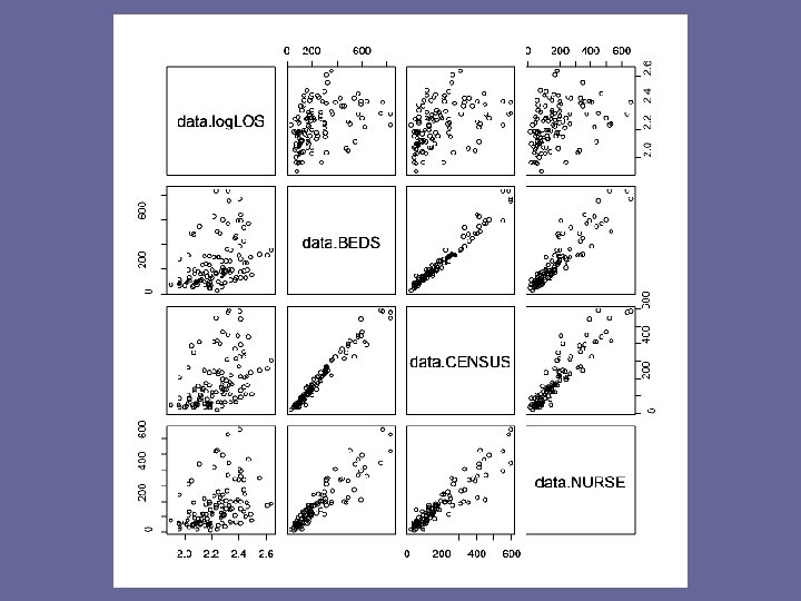
Example § Let’s look at our classic example of log. LOS § What variables are associated with log. LOS? § What variables have the potential to create multicollinearity?

SENIC

> > > data <- read. csv("senicfull. csv") data$log. LOS <- log(data$LOS) data$nurse 2 <- data$NURSE^2 data$ms <- ifelse(data$MEDSCHL==2, 0, data$MEDSCHL) data. cor <- data[, -1] > round(cor(data. cor), 2) LOS AGE INFRISK CULT XRAY BEDS MEDSCHL REGION CENSUS NURSE LOS 1. 00 0. 19 0. 53 0. 38 0. 41 -0. 30 -0. 49 0. 47 0. 34 AGE 0. 19 1. 00 0. 00 -0. 23 -0. 02 -0. 06 0. 15 -0. 02 -0. 05 -0. 08 INFRISK 0. 53 0. 00 1. 00 0. 56 0. 45 0. 36 -0. 23 -0. 19 0. 38 0. 39 CULT 0. 33 -0. 23 0. 56 1. 00 0. 42 0. 14 -0. 24 -0. 31 0. 14 0. 20 XRAY 0. 38 -0. 02 0. 45 0. 42 1. 00 0. 05 -0. 09 -0. 30 0. 06 0. 08 BEDS 0. 41 -0. 06 0. 36 0. 14 0. 05 1. 00 -0. 59 -0. 11 0. 98 0. 92 MEDSCHL -0. 30 0. 15 -0. 23 -0. 24 -0. 09 -0. 59 1. 00 0. 10 -0. 61 -0. 59 REGION -0. 49 -0. 02 -0. 19 -0. 31 -0. 30 -0. 11 0. 10 1. 00 -0. 15 -0. 11 CENSUS 0. 47 -0. 05 0. 38 0. 14 0. 06 0. 98 -0. 61 -0. 15 1. 00 0. 91 NURSE 0. 34 -0. 08 0. 39 0. 20 0. 08 0. 92 -0. 59 -0. 11 0. 91 1. 00 FACS 0. 36 -0. 04 0. 41 0. 19 0. 11 0. 79 -0. 52 -0. 21 0. 78 log. LOS 0. 98 0. 17 0. 55 0. 39 0. 42 -0. 32 -0. 52 0. 48 0. 37 nurse 2 0. 25 -0. 04 0. 26 0. 15 0. 04 0. 86 -0. 56 -0. 07 0. 84 0. 95 ms 0. 30 -0. 15 0. 23 0. 24 0. 09 0. 59 -1. 00 -0. 10 0. 61 0. 59 >

Let’s try an example with serious multicollinearity § To anticipate multicollinearity, ALWAYS good to look at scatterplots and correlation matrices of potential covariates § What covariates would give rise to a good example?