Interval Estimation of System Dynamics Model Parameters Spivak

Interval Estimation of System Dynamics Model Parameters Spivak S. I. – prof. , Bashkir State University Kantor O. G. – senior staff scientist, Institute of Social and Economic Research, Ufa Scientific Centre of RAS Salahov I. R. – post graduate student, Bashkir State University 1

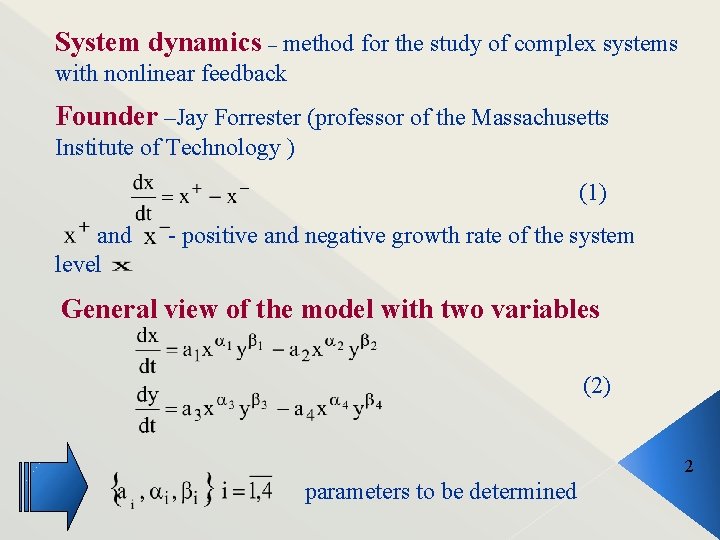
System dynamics – method for the study of complex systems with nonlinear feedback Founder –Jay Forrester (professor of the Massachusetts Institute of Technology ) (1) and level - positive and negative growth rate of the system General view of the model with two variables (2) 2 parameters to be determined

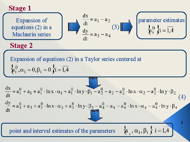
Stage 1 Expansion of equations (2) in a Maclaurin series (3) parameter estimates Stage 2 Expansion of equations (2) in a Taylor series centered at (4) 3 point and interval estimates of the parameters

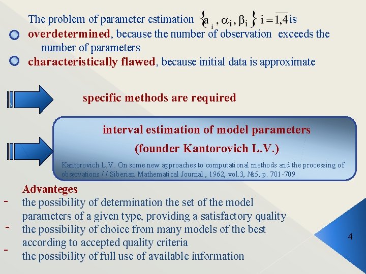
The problem of parameter estimation is overdetermined, because the number of observation exceeds the number of parameters characteristically flawed, because initial data is approximate specific methods are required interval estimation of model parameters (founder Kantorovich L. V. ) Kantorovich L. V. On some new approaches to computational methods and the processing of observations / / Siberian Mathematical Journal , 1962, vol. 3, № 5, p. 701 -709 - Advanteges the possibility of determination the set of the model parameters of a given type, providing a satisfactory quality the possibility of choice from many models of the best according to accepted quality criteria the possibility of full use of available information 4

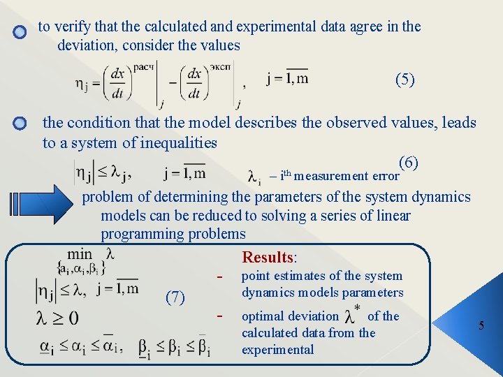
to verify that the calculated and experimental data agree in the deviation, consider the values (5) the condition that the model describes the observed values, leads to a system of inequalities (6) th – i measurement error problem of determining the parameters of the system dynamics models can be reduced to solving a series of linear programming problems (7) - Results: point estimates of the system dynamics models parameters optimal deviation of the calculated data from the experimental 5

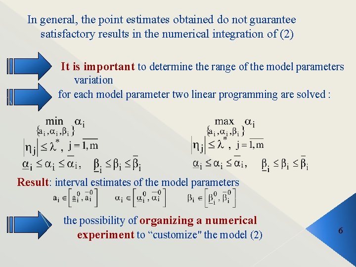
In general, the point estimates obtained do not guarantee satisfactory results in the numerical integration of (2) It is important to determine the range of the model parameters variation for each model parameter two linear programming are solved : Result: interval estimates of the model parameters the possibility of organizing a numerical experiment to “customize" the model (2) 6

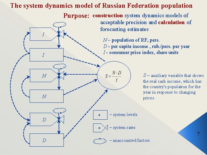
The system dynamics model of Russian Federation population Purpose: construction system dynamics models of I acceptable precision and calculation of forecasting estimates N – population of RF, pers. D - per capita income , rub. /pers. per year I - consumer price index, share units I S – auxiliary variable that shows N the real cash income, which has the country's population for the year in response to changing prices N D D * – system levels * – system rates 7 – unaccounted factors

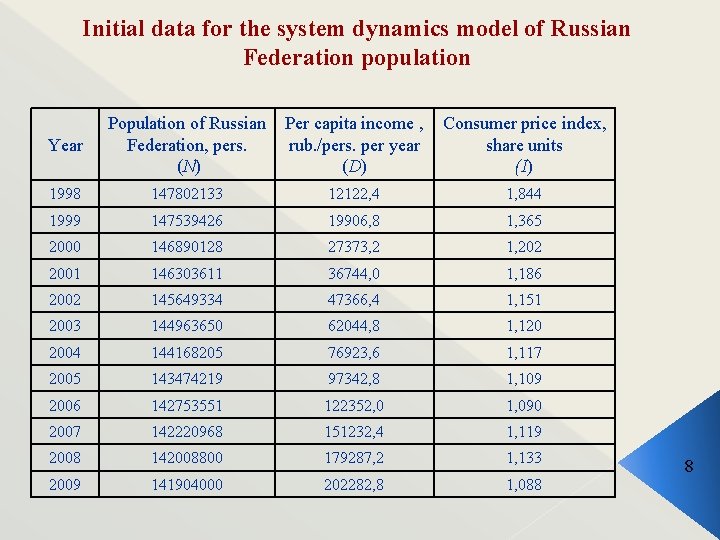
Initial data for the system dynamics model of Russian Federation population Year Population of Russian Federation, pers. (N) Per capita income , rub. /pers. per year (D) Consumer price index, share units (I) 1998 147802133 12122, 4 1, 844 1999 147539426 19906, 8 1, 365 2000 146890128 27373, 2 1, 202 2001 146303611 36744, 0 1, 186 2002 145649334 47366, 4 1, 151 2003 144963650 62044, 8 1, 120 2004 144168205 76923, 6 1, 117 2005 143474219 97342, 8 1, 109 2006 142753551 122352, 0 1, 090 2007 142220968 151232, 4 1, 119 2008 142008800 179287, 2 1, 133 2009 141904000 202282, 8 1, 088 8

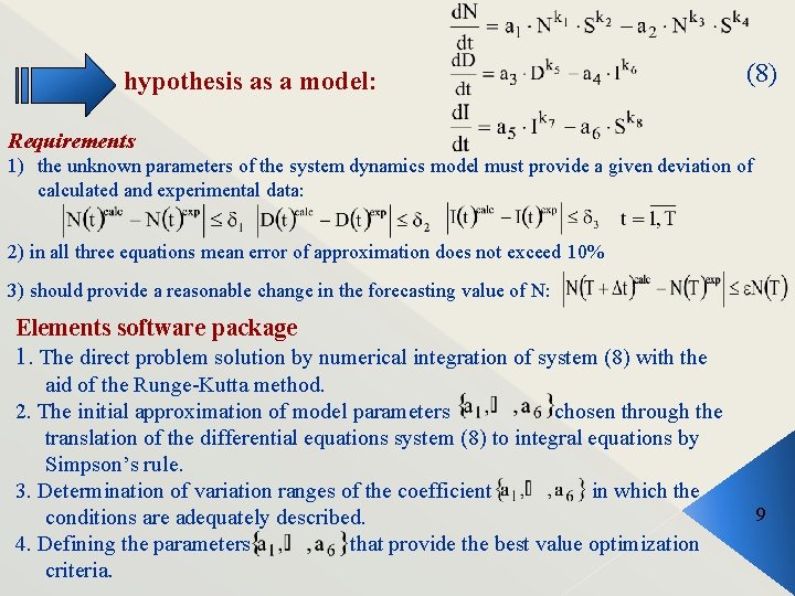
hypothesis as a model: (8) Requirements 1) the unknown parameters of the system dynamics model must provide a given deviation of calculated and experimental data: 2) in all three equations mean error of approximation does not exceed 10% 3) should provide a reasonable change in the forecasting value of N: Elements software package 1. The direct problem solution by numerical integration of system (8) with the aid of the Runge-Kutta method. 2. The initial approximation of model parameters chosen through the translation of the differential equations system (8) to integral equations by Simpson’s rule. 3. Determination of variation ranges of the coefficient in which the conditions are adequately described. 4. Defining the parameters that provide the best value optimization criteria. 9

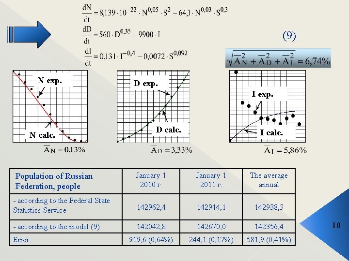
(9) N exp. D exp. I exp. N calc. D calc. I calc. January 1 2010 г. January 1 2011 г. The average annual - according to the Federal State Statistics Service 142962, 4 142914, 1 142938, 3 - according to the model (9) 142042, 8 142670, 0 142356, 4 919, 6 (0, 64%) 244, 1 (0, 17%) 581, 9 (0, 41%) Population of Russian Federation, people Error 10

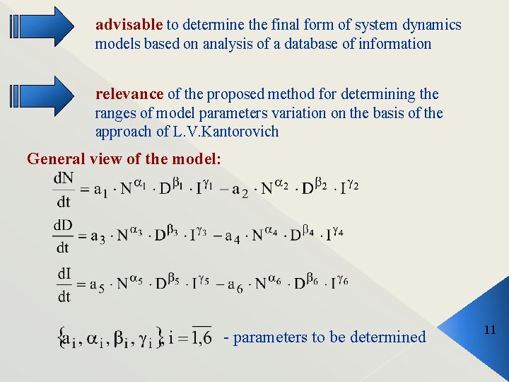
advisable to determine the final form of system dynamics models based on analysis of a database of information relevance of the proposed method for determining the ranges of model parameters variation on the basis of the approach of L. V. Kantorovich General view of the model: - parameters to be determined 11

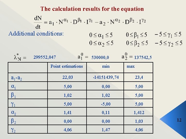
The calculation results for the equation Additional conditions: 299552, 047 530000, 0 137542, 5 Point estimations min max a 1 -a 2 22, 03 -14151439, 74 23, 4 α 1 5, 00 0, 00 5, 00 β 1 1, 02 5, 00 γ 1 5, 00 -5, 00 α 2 1, 41 0, 11 1, 412 β 2 0, 00 1, 03 γ 2 4, 06 1, 47 4, 06 12

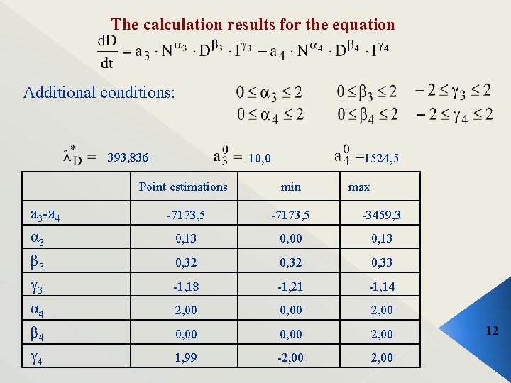
The calculation results for the equation Additional conditions: 393, 836 10, 0 1524, 5 Point estimations min -7173, 5 -3459, 3 α 3 0, 13 0, 00 0, 13 β 3 0, 32 0, 33 γ 3 -1, 18 -1, 21 -1, 14 α 4 2, 00 0, 00 2, 00 β 4 0, 00 2, 00 γ 4 1, 99 -2, 00 a 3 -a 4 max 12

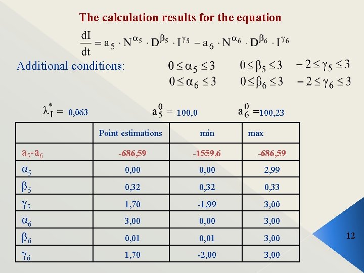
The calculation results for the equation Additional conditions: 0, 063 100, 0 100, 23 Point estimations min -686, 59 -1559, 6 -686, 59 α 5 0, 00 2, 99 β 5 0, 32 0, 33 γ 5 1, 70 -1, 99 3, 00 α 6 3, 00 0, 00 3, 00 β 6 0, 01 3, 00 γ 6 1, 70 -2, 00 3, 00 a 5 -a 6 max 12

Thank you 1