Intermediate Microeconomics WESS 16 FIRMS AND PRODUCTION Laura

Intermediate Microeconomics WESS 16 FIRMS AND PRODUCTION Laura Sochat

Production functions The labor (employees) and capital (factories, robots) a firm uses are called the factors of production, or inputs. The amount of goods and services produced are called the firm's output. Given a specific combination of inputs, the firm can produce a certain amount of outputs. – The production function tells us the maximum amount the firm can produce give a particular combination of inputs. – Assuming amount of capital used is denoted as K, amount of labor used as L, and quantity of output as Q, we can write the production function as: Q=f(L, K)

Marginal and average product

Relationship between Marginal and Average product 10 5 0 6 12 24 18 , -10 Q 6 30 5 12 96 8 18 162 9 24 192 8 30 150 5 L, 000 s man hour per day -5 L

Marginal and average product C B Total Product Function A 0 18 000 s man hour per day , 10 5 0 -5 18 24 000 s man hour per day , -10 The total product function single input production function depicting how output depends on the level of that input used, given a fixed amount of other inputs used. Law of diminishing marginal returns: Principle that as the usage of one input increases, the quantities of other inputs being held fixed, a point will be reached beyond which the marginal product of the variable input will decrease.

ISOQUANTS 0 6 12 18 24 30 0 0 0 6 0 5 15 25 30 23 L 12 0 15 48 81 96 75 18 0 25 81 137 162 127 24 0 30 96 162 192 150 30 0 23 75 127 150 117 K, 000 s of machine hour a day Isoquants enable us to represent the production function. It is a curve that shows all combinations of labor and capital that can produce a given level of output. A 18 B 6 6 18 L, 000 s of machine hour a day

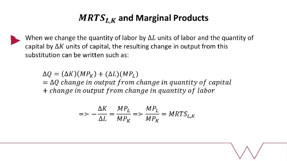
Marginal rate of Technical substitution The marginal rate of technical substitution (of labor for capital) is the rate at which capital can be reduced for every one unit increase in labor, and keeping output constant. It is defined as the absolute value of slope of the isoquant drawn with labor on the horizontal axis, and capital on the vertical axis. K, 000 s of machine hour a day 50 A B 20 20 50 L, 000 s of machine hour a day

Special production functions: Linear and fixed proportions production functions 10 Inputs are perfect complements Q, quantity of oxygen atoms H, High capacity computers Inputs are perfect substitutes A C 5 C B 10 20 L, Low capacity computers (a) Map of isoquants for data storing B 3 2 1 A 2 4 6 H, quantity of hydrogen atoms (b) Map of isoquants for molecules of water

K, units of capital per day Special production functions: Cobb Douglas production function 50 40 30 20 10 10 20 30 40 50 L, units of labor per day

Returns to scale

Returns to scale

K, units of capital per year The distinction between returns to scale and diminishing marginal returns • Returns to scale refer to the impact of an increase in all input quantities simultaneously • Marginal returns refer to an increase in the quantity of a single input, such as labor holding quantities of all other inputs fixed. E 30 D 20 A B 10 10 20 C 30 L, units of labor per year • The figure to the left illustrates a situation where there are diminishing marginal returns to labor, but constant returns to scale.

K, units of capital per year Neutral technological progress A 0 L, units of labor per year

Labor-saving technological progress K, units of capital per year A 0 L, units of labor per year

Capital saving technological progress K, units of capital per year L, units of labor per year