ICES ASC 2018 Q 452 Densitydependent growth in

ICES, ASC 2018, Q: 452 Density-dependent growth in North Atlantic fishes: exception or the rule? by Jan Horbowy*, Jeremy Collie**, Adrien Tableau** *National Marine Fisheries Research Institute, Gdynia, Poland **Afiliation to be inserted

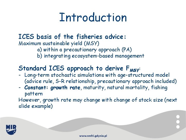
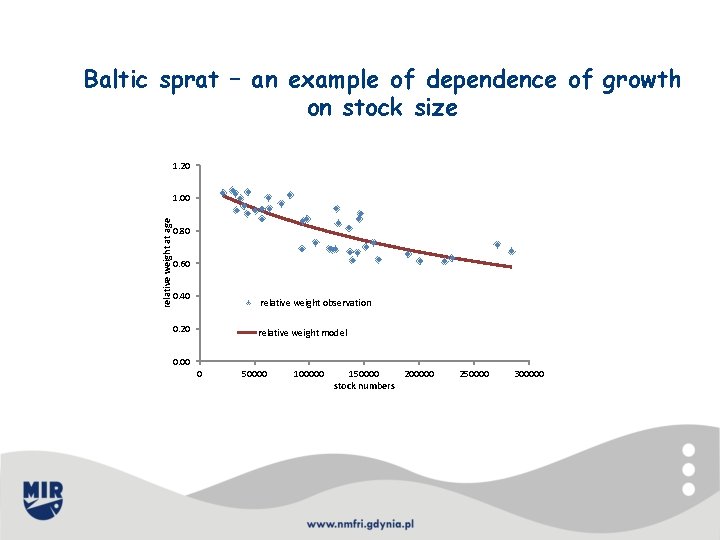
Introduction ICES basis of the fisheries advice: Maximum sustainable yield (MSY) a) within a precautionary approach (PA) b) integrating ecosystem-based management Standard ICES approach to derive FMSY: - Long-term stochastic simulations with age-structured model (advice rule, S-R relationship, precautionary approach included) - Constant: growth rate, maturity, natural mortality, fishing pattern However, growth rate may change with change of stock size (next slide example)

Baltic sprat – an example of dependence of growth on stock size 1. 20 relative weight at age 1. 00 0. 80 0. 60 0. 40 relative weight observation 0. 20 relative weight model 0. 00 0 50000 100000 150000 200000 stock numbers 250000 300000

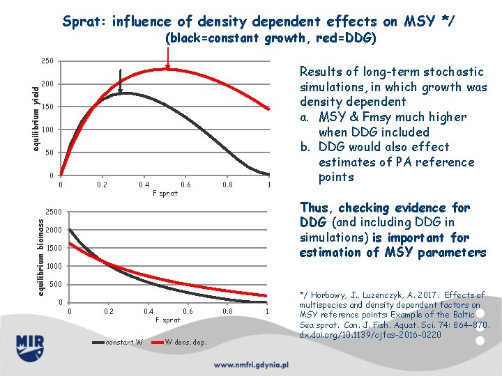
Sprat: influence of density dependent effects on MSY */ (black=constant growth, red=DDG) equilibrium yield 250 200 150 100 50 0 0 0. 2 0. 4 F sprat 0. 6 0. 8 1 Thus, checking evidence for DDG (and including DDG in simulations) is important for estimation of MSY parameters 2500 equilibrium biomass Results of long-term stochastic simulations, in which growth was density dependent a. MSY & Fmsy much higher when DDG included b. DDG would also effect estimates of PA reference points 2000 1500 1000 500 0 0 0. 2 0. 4 constant W F sprat 0. 6 W dens. dep. 0. 8 1 */ Horbowy, J. , Luzenczyk, A. 2017. Effects of multispecies and density dependent factors on MSY reference points: Example of the Baltic Sea sprat. Can. J. Fish. Aquat. Sci. 74: 864– 870. dx. doi. org/10. 1139/cjfas-2016 -0220

Stocks considered & Data 53 stock were analysed: - 43 stocks from European waters (mainly cod, haddock, saithe, whiting, herring, sole, plaice) -10 US stocks from north-west Atlantic (cod, haddock, flatfishes from Gulf of Main & Georges Bank) Data a. Weight at age data: from ICES WGs; where possible taken as WEST (weight in the stock) , otherwise WECA (weight in the catch) b. Biomass (TSB, SSB) and recruitment: most recent ICES assessment (2017 or 2018) c. USA data Jeremy please help

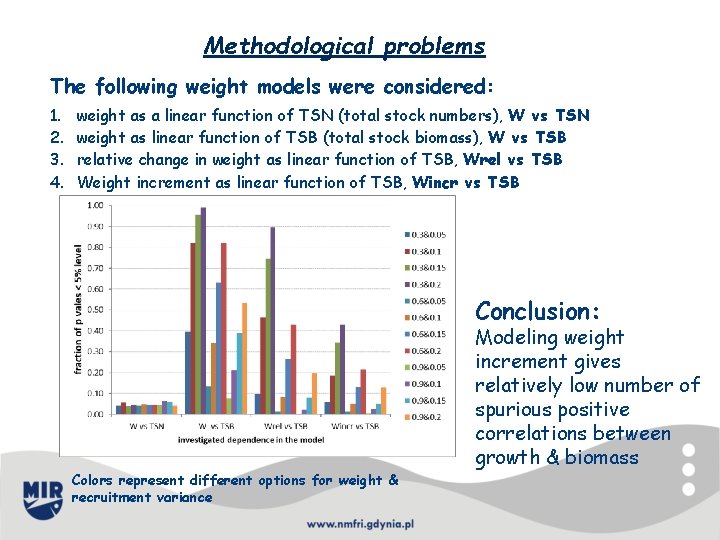
Methodological problems In simple statistical analysis of the type weight = function of biomass spurious correlations (positive) may occur as weight is present at both side of the above equation. It may be illustrated in simulations by: - generating random weights and random stock numbers (through random recruitment) - relating different measures of growth change with stock biomass.

Methodological problems The following weight models were considered: 1. 2. 3. 4. weight as a linear function of TSN (total stock numbers), W vs TSN weight as linear function of TSB (total stock biomass), W vs TSB relative change in weight as linear function of TSB, Wrel vs TSB Weight increment as linear function of TSB, Wincr vs TSB Conclusion: Modeling weight increment gives relatively low number of spurious positive correlations between growth & biomass Colors represent different options for weight & recruitment variance

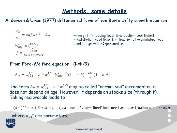
Methods, some details Andersen & Ursin (1977) differential form of von Bertalanffy growth equation w=weight, f=feeding level, h=anabolism coefficient, k=catabolism coefficient, v=fraction of assimilated food used for growth, Q=parameter. From Ford-Walford equation (K=k/3) (reciprocal of „normalised” increment as linear function of stock size)

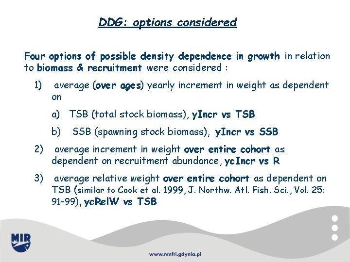
DDG: options considered Four options of possible density dependence in growth in relation to biomass & recruitment were considered : 1) average (over ages) yearly increment in weight as dependent on a) TSB (total stock biomass), y. Incr vs TSB b) SSB (spawning stock biomass), y. Incr vs SSB 2) average increment in weight over entire cohort as dependent on recruitment abundance, yc. Incr vs R 3) average relative weight over entire cohort as dependent on TSB (similar to Cook et al. 1999, J. Northw. Atl. Fish. Sci. , Vol. 25: 91– 99), yc. Rel. W vs TSB

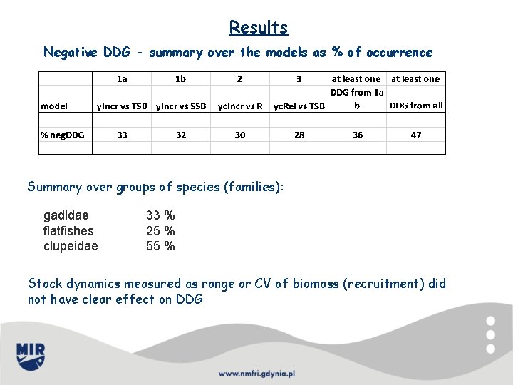
Results Negative DDG - summary over the models as % of occurrence Summary over groups of species (families): gadidae flatfishes clupeidae 33 % 25 % 55 % Stock dynamics measured as range or CV of biomass (recruitment) did not have clear effect on DDG

Results Other summaries Jeremy please help

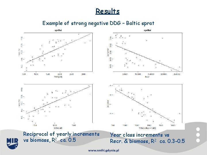
Results Example of strong negative DDG – Baltic sprat Reciprocal of yearly increments vs biomass, R 2 ca. 0. 5 Year class increments vs Recr. & biomass, R 2 ca. 0. 3 -0. 5

Conclusions 1. DDG occurs for quite big percentage of stock a) over 30% for given model b) almost 50% for at least one of the models 2. Next conclusion, Jeremy please help 3. Further investigation: testing other error structure in fitting the models (relevant here ? ? ? )

Thank you