Highresolution 3 D modelling of oceanic fine structures

High-resolution 3 D modelling of oceanic fine structures using vertically adaptive coordinates Hans Burchard 1, Ulf Gräwe 1, Richard Hofmeister 2, Peter Holtermann 1, Inga Hense 3 and Jean-Marie Beckers 4 1. Leibniz Institute for Baltic Sea Research Warnemünde, Germany 2. Helmholtz-Zentrum Geesthacht, Institute for Coastal Research, Germany 3. Clima. Campus, University of Hamburg, Germany 4. GHER, University of Liege, Belgium hans. burchard@io-warnemuende. de

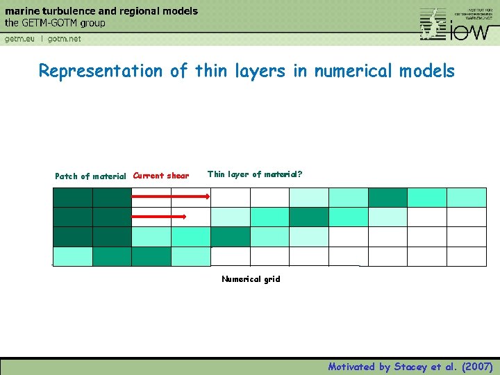
Representation of thin layers in numerical models Patch of material Current shear Thin layer of material? material Numerical grid Motivated by Stacey et al. (2007)

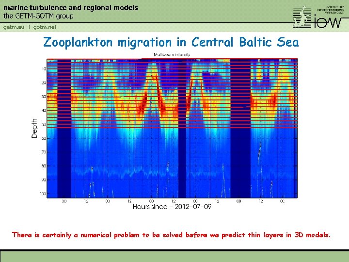
Zooplankton migration in Central Baltic Sea There is certainly a numerical problem to be solved before we predict thin layers in 3 D models.

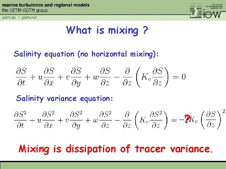
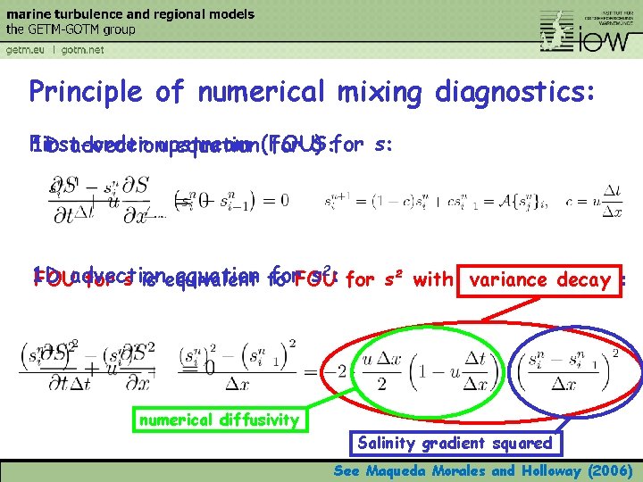
What is mixing ? Salinity equation (no horizontal mixing): Salinity variance equation: ? Mixing is dissipation of tracer variance.

Principle of numerical mixing diagnostics: First-order 1 D advectionupstream equation (FOU) for S: for s: 1 D equation to for. FOU s 2: for s² with variance decay : FOUadvection for s is equivalent numerical diffusivity Salinity gradient squared See Maqueda Morales and Holloway (2006)

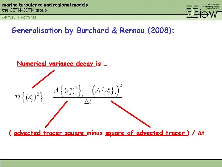
Generalisation by Burchard & Rennau (2008): Numerical variance decay is … ( advected tracer square minus square of advected tracer ) / Dt

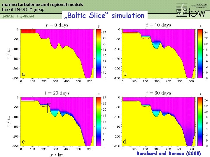
„Baltic Slice“ simulation Burchard and Rennau (2008)

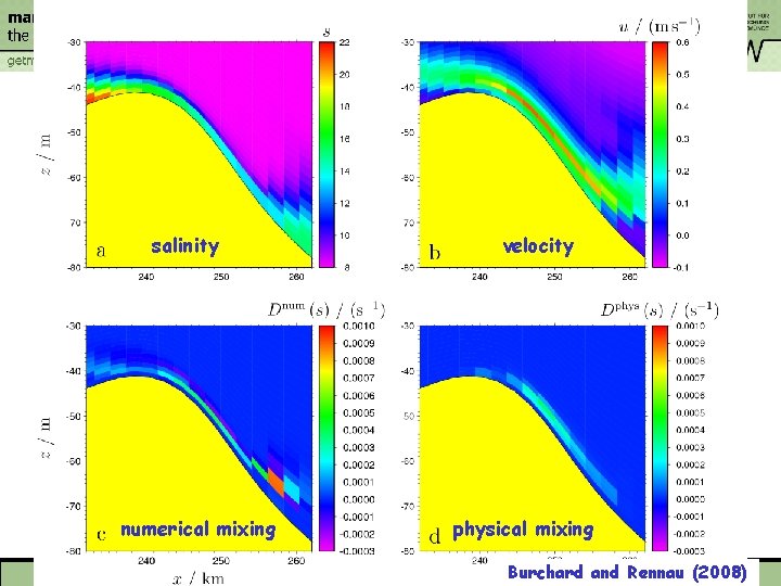
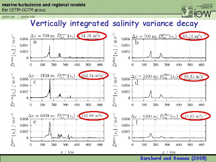
salinity numerical mixing velocity physical mixing Burchard and Rennau (2008)

Vertically integrated salinity variance decay Burchard and Rennau (2008)

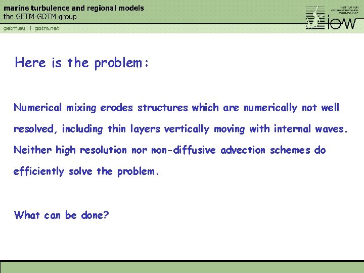
Here is the problem: Numerical mixing erodes structures which are numerically not well resolved, including thin layers vertically moving with internal waves. Neither high resolution nor non-diffusive advection schemes do efficiently solve the problem. What can be done?

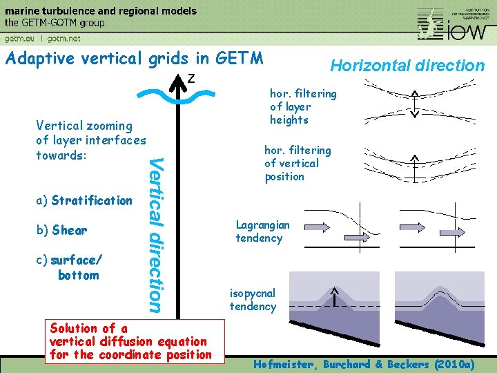
Adaptive vertical grids in GETM z a) Stratification b) Shear c) surface/ bottom Vertical direction Vertical zooming of layer interfaces towards: Solution of a bottom vertical diffusion equation for the coordinate position Horizontal direction hor. filtering of layer heights hor. filtering of vertical position Lagrangian tendency isopycnal tendency Hofmeister, Burchard & Beckers (2010 a)

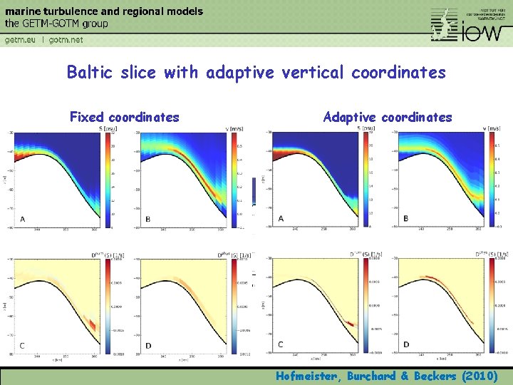
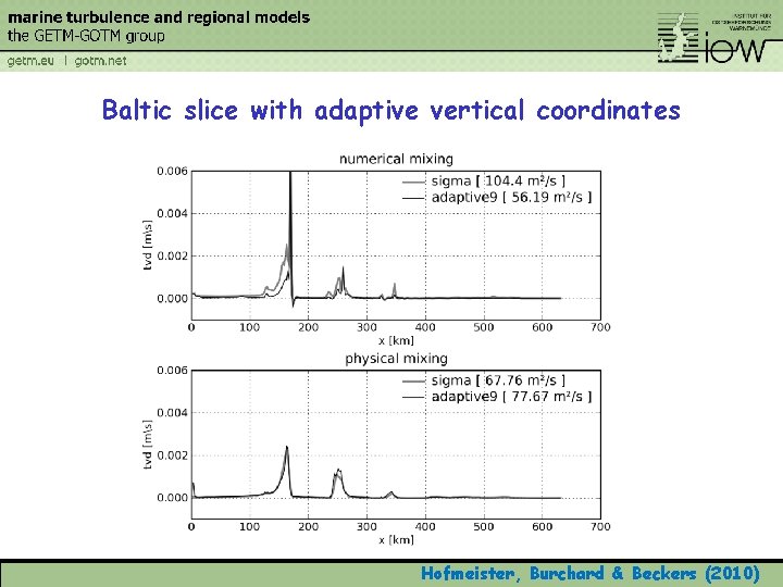
Baltic slice with adaptive vertical coordinates Fixed coordinates Adaptive coordinates Hofmeister, Burchard & Beckers (2010)

Baltic slice with adaptive vertical coordinates Hofmeister, Burchard & Beckers (2010)

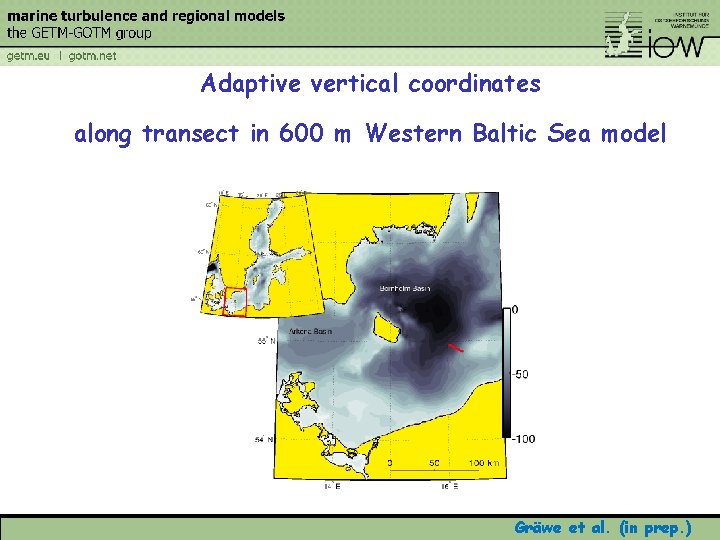
Adaptive vertical coordinates along transect in 600 m Western Baltic Sea model Gräwe et al. (in prep. )

Adaptive coordinates in Bornholm Sea

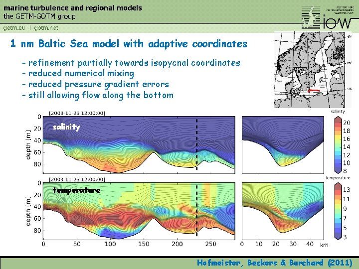
1 nm Baltic Sea model with adaptive coordinates - refinement partially towards isopycnal coordinates - reduced numerical mixing - reduced pressure gradient errors - still allowing flow along the bottom salinity temperature km Hofmeister, Beckers & Burchard (2011)

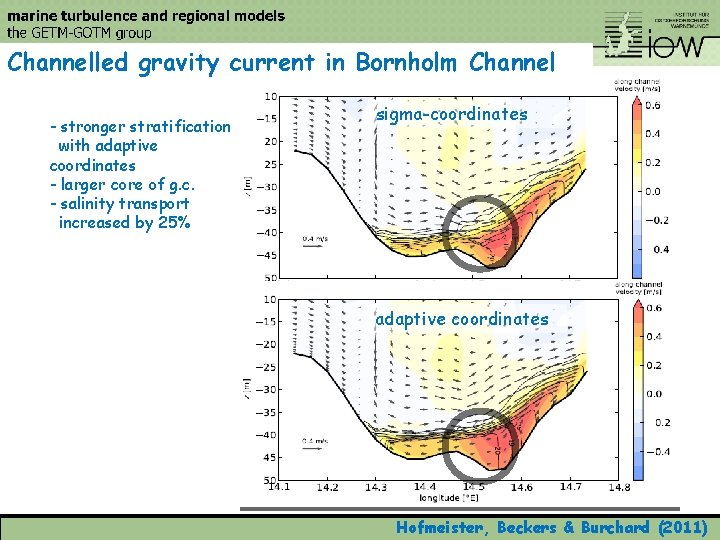
Channelled gravity current in Bornholm Channel - stronger stratification with adaptive coordinates - larger core of g. c. - salinity transport increased by 25% sigma-coordinates - interface jet along the coordinates adaptive coordinates Hofmeister, Beckers & Burchard (2011)

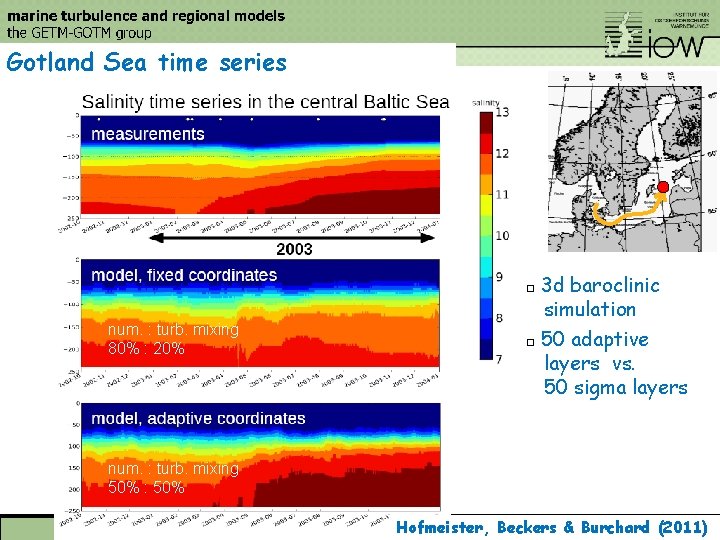
Gotland Sea time series 3 d baroclinic simulation � 50 adaptive layers vs. 50 sigma layers � num. : turb. mixing 80% : 20% num. : turb. mixing 50% : 50% Hofmeister, Beckers & Burchard (2011)

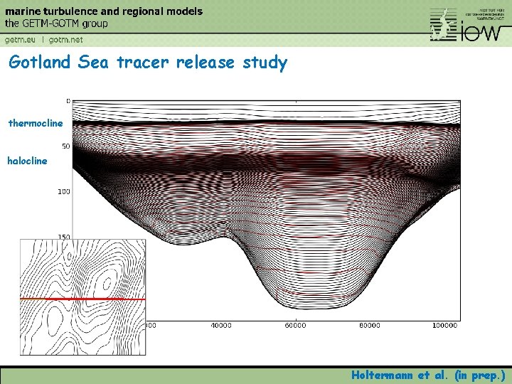
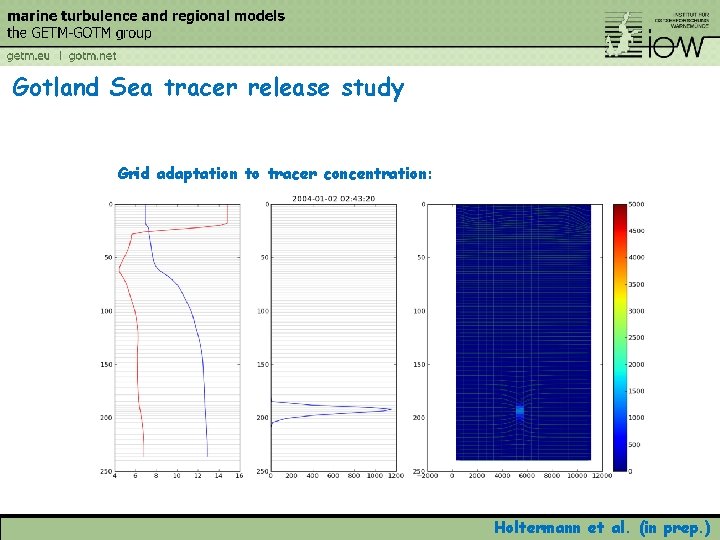
Gotland Sea tracer release study thermocline halocline Holtermann et al. (in prep. )

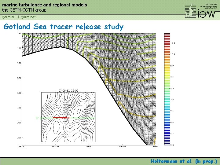
Gotland Sea tracer release study Holtermann et al. (in prep. )

Gotland Sea tracer release study Grid adaptation to tracer concentration: Holtermann et al. (in prep. )

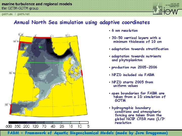
Annual North Sea simulation using adaptive coordinates • 6 nm resolution • 30 -50 vertical layers with a minimum thickness of 10 cm • adaptation towards stratification • adaptation towards nutrients and phytoplankton • production run 2005 -2006 • NPZD included via FABM • NPZD starts 2005 from uniform values • open boundaries for FABM are taken from a 1 D simulation of GOTM • hydrographic boundary conditions and atmospheric forcing are taken from the global NCEP CFSR runs (1/3 o resolution FABM = Framework of Aquatic Biogeochamical Models (made by Jorn Bruggeman)

Ada Temperature in S 1 [°C] phys & bio adaptive with 50 layers phys & bio adaptive with 30 layers phys adaptive with 30 layers non-adaptive with 30 layers Gräwe et al. (in prep. )

Layer thickness in S 1 [m] phys & bio adaptive with 50 layers phys & bio adaptive with 30 layers phys adaptive with 30 layers non-adaptive with 30 layers Gräwe et al. (in prep. )

Physical mixing in S 1 log 10[Dphy/(K 2/s)] phys & bio adaptive with 50 layers phys & bio adaptive with 30 layers phys adaptive with 30 layers non-adaptive with 30 layers Gräwe et al. (in prep. )

Numerical mixing in S 1 log 10[Dnum/(K 2/s)] phys & bio adaptive with 50 layers phys & bio adaptive with 30 layers phys adaptive with 30 layers non-adaptive with 30 layers Gräwe et al. (in prep. )

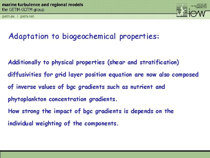
Adaptation to biogeochemical properties: Additionally to physical properties (shear and stratification) diffusivities for grid layer position equation are now also composed of inverse values of bgc gradients such as nutrient and phytoplankton concentration gradients. How strong the impact of bgc gradients is depends on the individual weighting of the components.

Nutrients at S 1 [mmol N/m 3] phys & bio adaptive with 50 layers phys & bio adaptive with 30 layers phys adaptive with 30 layers non-adaptive with 30 layers Gräwe et al. (in prep. )

Phytoplankton at S 1 [mmol N/m 3] phys & bio adaptive with 50 layers phys & bio adaptive with 30 layers phys adaptive with 30 layers non-adaptive with 30 layers Gräwe et al. (in prep. )

Phytoplankton at S 1 log 10[P/(mmol N/m 3)] phys & bio adaptive with 50 layers phys & bio adaptive with 30 layers phys adaptive with 30 layers non-adaptive with 30 layers Gräwe et al. (in prep. )

Zooplankton at S 1 [mmol N/m 3] phys & bio adaptive with 50 layers phys & bio adaptive with 30 layers phys adaptive with 30 layers non-adaptive with 30 layers Gräwe et al. (in prep. )

Detritus at S 1 [mmol N/m 3] phys & bio adaptive with 50 layers phys & bio adaptive with 30 layers phys adaptive with 30 layers non-adaptive with 30 layers Gräwe et al. (in prep. )

Temperature along T 1 [°C] phys & bio adaptive with 50 layers phys & bio adaptive with 30 layers phys adaptive with 30 layers non-adaptive with 30 layers Gräwe et al. (in prep. )

Physical mixing along T 1 log 10[Dphy/(K 2/s)] phys & bio adaptive with 50 layers phys & bio adaptive with 30 layers phys adaptive with 30 layers non-adaptive with 30 layers Gräwe et al. (in prep. )

Nutrients along T 1 [mmol N/m 3] phys & bio adaptive with 50 layers phys & bio adaptive with 30 layers phys adaptive with 30 layers non-adaptive with 30 layers Gräwe et al. (in prep. )

Phytoplankton along T 1 [mmol N/m 3] phys & bio adaptive with 50 layers phys & bio adaptive with 30 layers phys adaptive with 30 layers non-adaptive with 30 layers Gräwe et al. (in prep. )

Zooplankton along T 1 [mmol N/m 3] phys & bio adaptive with 50 layers phys & bio adaptive with 30 layers phys adaptive with 30 layers non-adaptive with 30 layers Gräwe et al. (in prep. )

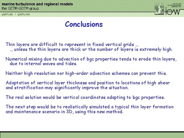
Conclusions Thin layers are difficult to represent in fixed vertical grids … … unless the thin layers are thick or the number of layers is extremely high. Numerical mixing due to advection of bgc properties tends to erode thin layers, due to internal waves and tides. Neither high resolution nor high-order advection schemes can prevent this. Adaptation of vertical layer thickness and position to locations of high shear and stratification may significantly improve the situation. The real solution would be vertical coordinates adapting to bgc properties. The next step would be to realistically simulated a typical thin layer formation and maintenance scenario in 3 D, using this new method.