Highresolution modelling in mountainous areas MAP results Evelyne

High-resolution modelling in mountainous areas: MAP results Evelyne Richard Laboratoire d’Aérologie CNRS / Univ. Paul Sabatier Toulouse, France

What are the skills of high-resolution models to forecast orographically influenced precipitation? Does explicit (versus parameterized) convection lead to a gain in predictability? IOP 2 a – 17 September 1999 A short, intense, isolated, convective event 70 mm within 12 hours Sensitivity experiments performed with Meso-NH

MAP IOP 2 a: IR Meteosat

MAP target area

Composite radar reflectivity @ z = 2 km MAP – IOP 2 A 19: 00 UT 20: 00 UT 250 km 18: 00 UT 21: 00 UT 22: 00 UT 23: 00 UT

Observation Simulation (Δx =2 km) Toce Ticino watershed 20: 00 UT 23: 00 UT Reflectivity @ 2000 m

RADAR SIMULATION ECMWF: OP. ANA 1999 12 hour accumulated precipitation

Composite radar reflectivity @ z = 2 km 18: 00 UT 19: 00 UT 20: 00 UT 250 km 17: 00 UT Z > 60 d. Bz

Radar Retrieval (S-Pol) Simulation (Meso-NH) 12 km 18: 00 UT 19: 00 UT 20: 00 UT (x) hail + graupel hail (o) hail rain 100 km

Great ! My model is doing a good job

RADAR OBSERVATIONS ECMWF: OP. ANA 1999 MAP - IOP 2 A: Intense Convection Strong sensitivity to initial state Low predictability ARPEGE: OP. ANA. 1999 ECMWF: REANALYSIS ECMWF: OP. ANA. 2002

IOP 2 a ANA. OP. 1999 REANALYSIS REANA (NO MAP DATA) 850 h. Pa water vapor mixing ratio : 17 September 1999 12 UTC

MAP IOP 2 a Lascaux et al. , 2004 Streamlines at 1000 m, 17/09/99 12 UTC ECMWF ANALYSIS Low-level convergence between the Ligurian and Adriatic flows MAP ECMWF REANALYSIS Increase in the model resolution -> higher mountains -> the Ligurian flow is blocked

Prectitability ? Still a long way to go !

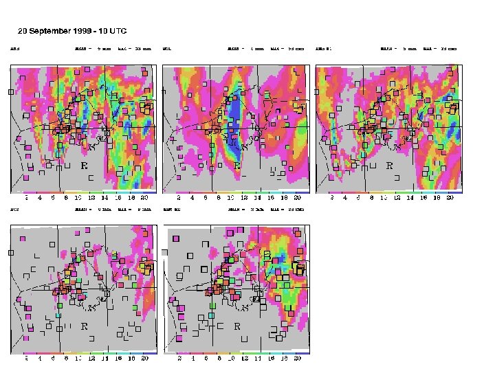
How do the models compare with each other ? IOP 2 b 20/21 September 1999: Orographic enhancement of a frontal system 200 mm within 30 h Model intercomparison : MC 2, MM 5, MOLOCH, Meso-NH

19 Sept. 1999 12: 00 METEOSAT infrared 20 Sept. 1999 12: 00

Sensitivity to the analysis ECMWF Op. Analysis Max: 512 mm Mean: 78 mm MAP Reanalysis Max: 482 mm Mean: 87 mm

The different models: • MESO-NH 10 KM + 2. 5 KM • MOLOCH 10 KM + 2 KM • MM 5 -RE 27 KM + 9 KM + 3 KM • MM 5 -E 1 18 KM + 6 KM + 2 KM • MC 2 +2 KM 40 KM + 10 KM Initial and boundary conditions from ECMWF operational analyses From 19 Sep. 12 UTC to 20 Sep. 18 UTC (30 hours)

Toce-Ticino watershed MAP - IOP 2 B - 19 -20 Sep. 1999 Intercomparison exercise 4 non-hydrostatic models with horizontal resolution of 2 to 3 km Initialization based upon ECMWF operational analysis Accumulated precipitation from the 19 th 15 UTC to the 20 th 18 UTC

Time evolution of the mean hourly precipitation rate Rain gauges Radar

Time evolution of the correlation coeffecient (wrt rain gauges)

Heidke skill scores as a function of precip. class 1 h precip. 27 h precip.

Comparison with rain gauge measurements (121 points)

Hydrological response Toce watershed 1532 km 2

Grossi et al. , 2004

Grossi et al. , 2004

How does the flow over complex terrain modify the growth mechanisms of precipitation particles? Three Doppler radars Monte Lema – Ronsard – S Pol Ronsard • Dual Doppler analysis • 3 D wind fields rerievals • Microphysical retrievals

Blocked and stable case dry snow U/Nh < 1 wet snow light rain Unblocked and unstable case graupel U/Nh > 1 riming coalescence heavy rain Medina and Houze, 2003

To what extend the models able to reproduce this contrasted behaviour in the microphysics ?

Mean vertical distribution of the hydrometeors IOP 2 A IOP 8 Ice Snow Graupel Snow Hail Cloud Rain IOP 2 a ( Strong convection) - Deep system -Large amount of hail and graupel IOP 8 ( Stratiform event) - Shallow system - Large amount of snow

Dominant microphysical processes: IOP 2 a Growth of graupel by RIMING DEPOSITION on ice (and sublimation) Depletion of graupel by WET GROWTH of hail IOP 8 ACCRETION of cloud droplets by raindrops MELTING-CONVERSION of the snow (into graupel) AUTOCONVERSION of pristine ice

Conclusion: IOP 2 A (Predictability) The use of non-hydrostatic high-resolution models will improve the precipitation forecast but only to some extend. Further improvement is tied to the improvement of the model initial state Adding mesoscale data in a global assimilation system is insufficient • Mesoscale data assimilation system • Limited area ensemble forecast (MAP D-PHASE)

n IOP 2 b (Model Intercomparison) – Very good consistency of the accumulated precipitation pattern – Model results over/under estimate the total precipitation by a factor ranging from +30% to -30% – The accuracy of the model precipitation is rather weak for the hourly rainfall but fairly reasonable for the precipitation accumulated over the 30 h time period of the event – However model results are not yet accurate enough to be used for hydrological forecast on small watersheds

Explicit microphysical schemes do provide fairly realistic results … The contrasted microphysical behaviour between different IOPs is reasonably reproduced • Convective – flow over ----> Strong riming and coalescence • Stratiform – blocked flow ----> Melting of snow

http: //www. aero. obs-mip. fr/map/MAP_wgnum N. Asencio (2), R. Benoit (3), A. Buzzi (4), R. Ferretti (5), F. Lascaux (1), P. Malguzzi (4), S. Serafin (6), G. Zängl (7), J-F. Georgis (1), R. Ranzi (8), G. Grossi (8), N. Kouwen (9) (1) LA CNRS/UPS, Toulouse, France (2) CNRM, Météo-France, Toulouse, France (3) RPN, Montréal, Canada (4) ISAC, CNR, Bologna, Italy (5) University of L ’Aquila, Italy (6) University of Milano, Italy (7) University of Munich, Germany (8) University of Brescia, Italy (9) University of Waterloo, Canada