Fragmented Credit Market Adverse Selection Adverse Selection arises

Fragmented Credit Market – Adverse Selection

• Adverse Selection arises due to a kind of information Asymmetry. • It has received a great deal of attention in the credit market • There is a great deal of heterogeneity among farmers in a village. While the lenders have a good idea about the average characteristics of the pool of the potential borrowers , they may not have complete information concerning the characteristics of any particular borrower. • This leads to problems of adverse selection

Model Specifications- Assumptions • Suppose that farming requires no effort, but that there are two types of potential borrowers indexed by t<- {I, 2}. Type 2 borrowers have access to land that is riskier but potentially more lucrative than that used by type 1 borrowers; that is • Expected Return to farming each type of land is identical Also suppose that the reservation utility of the different types of borrower is constant. The expected utility of a borrower is and the expected return from a loan at rate i to a type t borrower is

Competitive equilibrium with complete information • As a benchmark, we first assume that perfectly informed lenders compete to make loans within the village. Lenders can distinguish between the types of borrower, so they can offer different interest rates to each type. An equilibrium with lending to borrower type t will be an interest rate such that (c) there is no interest rate i(t) that yields are turn greater than or equal top to a lender and which a type t borrower would prefer to i 1(t). If there is an equilibrium with lending , it is characterized by solving for each t

Suppose that the lenders in the competitive credit market cannot differentiate between borrowers of different types, though they know the relative proportions of type 1 and type 2 farmers in the village. First, note that, at any given interest rate i; So safer borrowers achieve a lower expected utility from a given interest rate, but provide higher expected income to the lender. These results follow directly from the limited liability nature of the credit contract, which limits the loss faced by a borrower when her crop fails. Recall that the participation constraint is

ØDefine i*(l) as the highest interest rate at which type 1 borrowers are willing to borrow. So i*(1) is implicitly defined by the equation. ØDefine i*(2) analogously. i*(l) < i*(2) , so, as the interest rate increases, households with safer projects drop out of the pool of borrowers first. For interest rates less than i*(l), all potential borrowers demand credit. If the interest rate increases past i*( 1), the relatively safe type 1 borrowers stop demanding credit, while type 2 borrowers continue to demand loans. ØAs the safer borrowers drop out of the market, lender income falls discontinuously.

Figure illustrates the relationship between the interest rate charged by lenders and the expected income from lending. Lender income rises with increases in the interest rate until i = i*(l). Suppose p(l) is the proportion of the population of potential borrowers who are type 1. Then the expected income from a loan at interest i<= i*(1) is E ∏(i) = p(1)∏(1) i + [1 -p(1)] ∏(2) i. As i increases past i*(l), type 1 borrowers drop out of the market and lender income falls. As the interest rate continues to increase, lender income once again increases until i*(2), at which point type 2 borrowers stop demanding credit and no loans are made.

Definition – Comp. Eq. in adverse selection • Lenders cannot distinguish between borrowers of different types. Therefore, the competitive equilibrium with adverse selection is defined as an interest rate such that In other words, an interest rate i is an equilibrium interest rate if lenders do not lose money on average at i, and if there is no other interest rate which any type of borrower would prefer at which lenders would avoid losing money. There are no explicit borrower participation constraints in this definition of equilibrium because these constraints are built into the function E ∏(i).

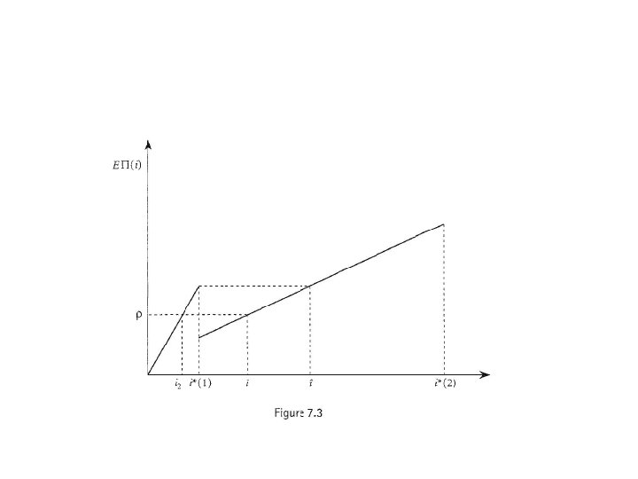
As long as R-p > W, (the condition for lending to be possible in the case of complete information), there will be lending in the equilibrium with adverse selection. ØIf p> E ∏(i *1) then the equilibrium interest rate will be an only the risky type 2 borrowers will demand loans. ØIf (as in Figure 7. 3), then the interest rate will be , which is less than i*(1), and all potential borrowers will demands loans. It should be clear that i is not an equilibrium ØAt that interest rate only risky borrowers would demand credit and lenders would make zero profits. But all borrowers

Many discussions of the implications of adverse selection for credit markets in less developed countries focus on the possibility of credit rationing. In this simple model, credit rationing does not occur. How does this model differ from the celebrated work of Stiglitz and Weiss (1981), which is theoretical basis of the worry that credit rationing might be pervasive? The essential difference is that the current model presumes that lenders have access to an infinitely elastic supply of funds at a cost of p. Figure illustrates the Stiglitz-Weiss result. The demand for loans is simply N 1+ N 2 for i<=i*(1), N 2 for i*(1) < i<=i*(2), and 0 for larger i, where Ni , is the number of the ith type of borrower.

ØWe have drawn this schedule so that rationing would occur in Equilibrium. Credit Rationing would occur The competitive equilibrium entails lenders charging i*(l) and earning an expected return EII(i*(l)). the demand for loans at i*(l) exceeds the supply of loanable funds, leading to a rationing of credit.

• An increase in the interest rate would cause type 1 borrowers to drop out of the market, leaving lenders with a riskier portfolio of loans and reducing expected returns to lending. At interest rate ie loan supply equals loan demand (with only type 2 borrowers in the market), but lenders earn a lower expected return than at i*(l): a lender charging i*(l) could attract borrowers of all types, and would earn a higher expected return. • In a manner exactly analogous to that discussed in Section II(a), the existence of collateral can eliminate the problem of adverse selection. As in that case, a pledge of collateral equal in value to the repayment owed by the borrower places the entire risk of the transaction on the borrower. The return to the lender no longer depends on the unknown type of the borrower, hence adverse selection no longer exists. • Once again , this result depends crucially on the assumed risk neutrality of the borrower. If the borrower is risk-averse, collateral can mitigate but not eliminate the consequences of adverse selection.

Equilibrium with a fully informed monopolist • Let us return to the case of a village with a monopolistic, omniscient moneylender. He knows which villagers have access to which type of land. As before, we assume that his opportunity cost of funds is p. • His problem is to set an interest rate i 3( t) for each type of borrower to solve: As long as R –p>= W, the equilibrium will involve lending to each type of borrower at interest rates i 3 ( t)(R -W)/∏( t) = i*( t). Each type of borrower achieves an expected utility of W, and the lender earns an expected return of R-p>=W on each loan.

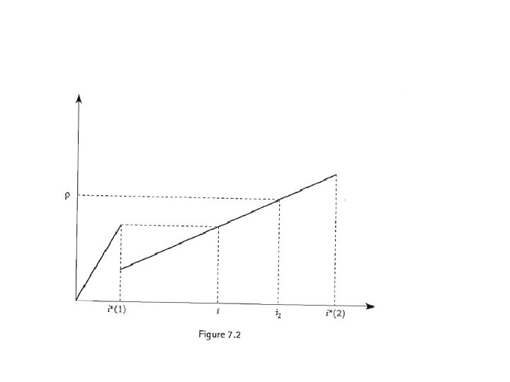
Competition between an informed local money lender and uninformed outside lenders • Once again, suppose that there is an active, competitive market for credit from lenders not resident in the village. These lenders cannot distinguish between type 1 and type 2 farmers. • They compete with a resident moneylender who knows the type of each farmer in the village. All lenders face an opportunity cost of funds equal to p. As in the case of moral hazard, the resident moneylender will be able to use his informational advantage to collect rents even in the face of this competitive pressure from uninformed lenders. • There are two cases to consider. First, suppose that E ∏(i*(1)) <p<=R -W (as in Figure 7. 2). The equilibrium with competitive, uninformed lenders would involve lending only to type 2 borrowers, with i 2 =p/ ∏(2). The local moneylender can charge different interest rates to different types of borrower; denote the interest charged by the local lender by i 4(t). • The availability of these outside loans to type 2 borrowers implies that the local moneylender cannot charge more than i 2 to type 2 farmers; so i 4 (2) = p/∏(2). • Type 1 farmers have no access to credit from outside lenders in this case; so the local lender can revert to his case monopoly behaviour for this type of farmer and set i 4(1 ) =(R -W)/ ∏(1 )=∏ *(1). • The local lender earns rent on his loans to type 1 borrowers (his return on these loans is R-W> p) because of his superior information.

• • • v Alternatively, suppose that p <= E ∏(i*(l)). In this case, the equilibrium with competitive uninformed lenders would involve outside lenders setting i 2<= i*(1) and lending to both types of farmer. The local moneylender can lend to type 1 farmers at any interest rate less than or equal to i 2. Suppose the local lender sets i 4 (1) = i 2 (or just a bit below). Some(all) of the type 1 borrowers would not borrow from the outside lender, but instead would borrow from the local lender. The outside lenders would be faced with a riskier pool of borrowers at i =i 2 than they had in case 2 with no local lender. Their expected return from loans at i 2 would fall below p. Outside lenders, therefore, cannot offer loans at interest rate i 2 • All type 1 borrowers will borrow from the local moneylender at i 4(1) = i 2 , and the outside lenders will lend at to type 2 borrowers only. The local moneylender will set i 2 (2) =. The local lender again earns his rents on his loans to type 1 borrowers (His return on these loans is because of the power provided to him by his superior information concerning the characteristics ofvillage residents.