Evolutionary Computational Intelligence Lecture 9 Noisy Fitness Ferrante

Evolutionary Computational Intelligence Lecture 9: Noisy Fitness Ferrante Neri University of Jyväskylä

Real world optimization problems l l Many real world optimization problems are characterized by uncertainties This means that the same solutions takes different fitness values on the basis of the time when it is calculated

Classification of uncertainties l l Uncertainties in optimization can be categorized into three classes. Noisy fitness function Approximated fitness function Robustness

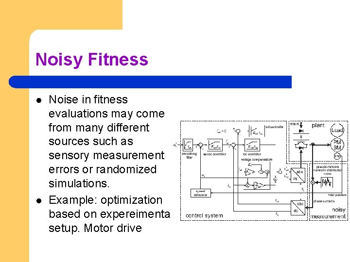
Noisy Fitness l l Noise in fitness evaluations may come from many different sources such as sensory measurement errors or randomized simulations. Example: optimization based on expereimental setup. Motor drive

Approximated Fitness Function l l When the fitness function is very expensive to evaluate, or an analytical fitness function is not available, approximated fitness functions are often used instead. These approximated models implicitly introduce a noise which is the difference between the approximated value and real fitness value, which is unknown.

Perturbation in the environment l l Often, when a solution is implemented, the design variables or the environmental parameters are subject to perturbations or changes Example satellite problem: due to the movement of the earth we are having some changes in the fitness values of the same solution

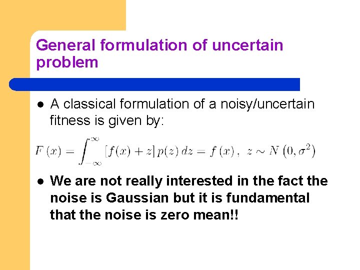
General formulation of uncertain problem l A classical formulation of a noisy/uncertain fitness is given by: l We are not really interested in the fact the noise is Gaussian but it is fundamental that the noise is zero mean!!

Zero mean: Explicit Averaging l l If the noise is zero mean, it is true that the average over a certain number of samples generates a ”good” estimation of the actual fitness values Thus, the most classical approach tends to compute the fitness each solution a certain number of times (samples) and then calculate the average

Failing of deterministic algorithms l l The noise introduces some ”false optima” in the fitness landscape and obviously a method which employs implicit or explicit information about the gradient can likely fail The estimation of the neighborhood cannot be properly done because the search is misled by the noise

Better success of EAs l l Evolutionary algorithms, due to their inner structure, so not perform comparison among neighbors and thus showed to be better performing in noisy environment Some recent papers are in fact stating that even rather standard EAs (e. g. self-adaptive ES) can lead to good results in noisy environment

Not universal success of EAs l l l This success is only restricted to specific cases and it strongly depends on the problem under examination EAs, like all the optimization algorithms, contain some comparison amongst solutions in order to determine which one is better and which one is worse In EAs this role is given to parent and survivor selection

Population based: Implicit Averaging l l EAs are population based algorithms thus another kind of averaging can be carried out Many scientists observed that large population size is efficient in defeating the noise since it is given a chance to calculate several neighbor solutions and thus detect promising areas

Another kind of averaging l l l Explicit and Implicit Averaging are in the class of averaging over the time Branke proposed averaging over the space: to calculate the fitness by averaging over the neighborhood of the point to be evaluated Implicit assumption: the noise in the neighborhood has the same characteristics as the noise at the point to be evaluated, and that the fitness landscape is locally smooth. This is not always true!!! E. g. systems with instable regions

High computational cost l l It is clear that an averaging operation (most of all over the time), requires extra fitness evaluations and thus an increase of computational overhead In some cases, in order to have reliable results it is necessary to spend a lot of efforts

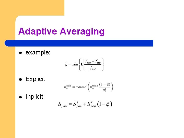
Adaptive Averaging l example: l Explicit l Inplicit

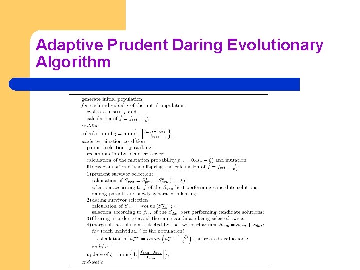
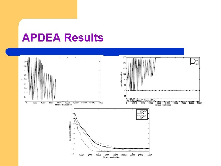
Prudent-daring survivor selection l l If not the individuals are re-sampled I can apply Two cooperative selection schemes – – l Prudent: selects individuals which are reliable (resampled) and fairly promising Daring: selects individuals which are unreliable (fitness calculated only once) but look very promising Reliable solution + computational saving

Adaptive Prudent Daring Evolutionary Algorithm

APDEA Results

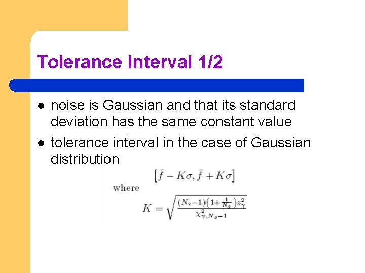
Tolerance Interval 1/2 l l noise is Gaussian and that its standard deviation has the same constant value tolerance interval in the case of Gaussian distribution

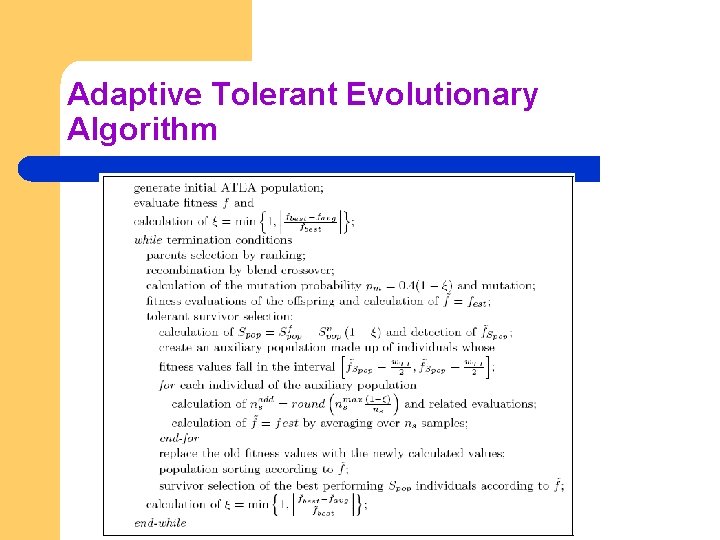
Tolerance Interval 2/2 l l If solution A is better than B of quantity equal to the half of the width of the tolerance interval, it is surely better (with a certain confidence level) If the distance in the fitness is smaller, then a re-sampling is required

Adaptive Tolerant Evolutionary Algorithm

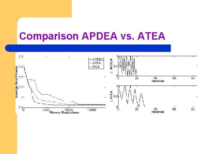
Comparison APDEA vs. ATEA

Comparative analysis l l APDEA is more general since it requires only that the noise is zero mean APDEA is better performing in terms of convergence velocity ATEA requires a preliminary analysis APDEA requires a more extensive parameter setting