Noisy Global Function Optimization Dan Lizotte Noisy Function

Noisy Global Function Optimization Dan Lizotte
 is a sample from P(F|x)")
Noisy Function? • Conditional distribution • Function ‘Evaluation’ F(x) is a sample from P(F|x) • There is no P(x) • We get to pick x, deterministically or stochastically, as usual.
 ~ µ(x) + ε(x) • What they don’t tell you:")
Common Assumptions • F(x) ~ µ(x) + ε(x) • What they don’t tell you: • µ(x) ‘arbitrary’ deterministic function • ε(x) is a r. v. , E(ε) = 0, (i. e. E(F(x)) = µ(x)) • Really only makes sense if ε(x) is unimodal • Samples are probably �� close to µ� • But maybe not normal
")
What’s the Difference? • Deterministic Function Opti�mization • Oh, I have this function f(x) • Gradient is ∇f… • Hessian is H… • Noisy Function Optimization • Oh, I have this r. v. F(x) ~ µ(x) + ε(x) • I think the form of µ is like… • I think that P(ε(x)) ~ something…
 ~ µ(x) + ε(x) • Estimate")
What’s the Plan? • Get samples of F(x) ~ µ(x) + ε(x) • Estimate and minimize µ(x) • Regression + Optimization • i. e. , reduce to deterministic global minimization
 Approach • Maybe I’m being unfair • Not claiming all non-Bayesians")
Frequentist (? ) Approach • Maybe I’m being unfair • Not claiming all non-Bayesians would think this is a good idea • Raises interesting questions
 ~ µ(x) + ε You")
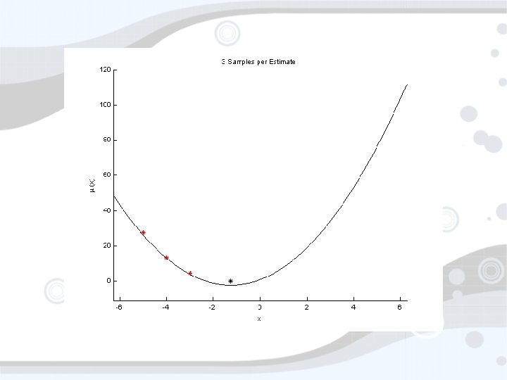
Suppose for a moment… • • You thought F(x) ~ µ(x) + ε You thought µ(x) = ax 2 + bx + c You thought ε ~ N(0, σ2) What do you do? • Estimate a, b, c • Minimize µ(x) (return xmin = -b/2 a) • Estimate how? • Sample points, do least squares (max L) • Sample where? Does it matter?
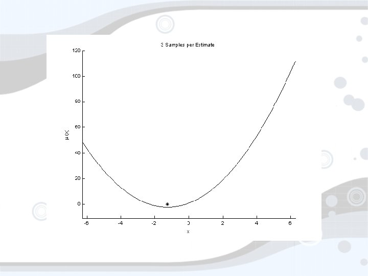

xmin=-1. 25 Std. Dev = 5. 77, Mean = -0. 22

xmin=-1. 25 Std. Dev = 0. 078, Mean = -1. 23

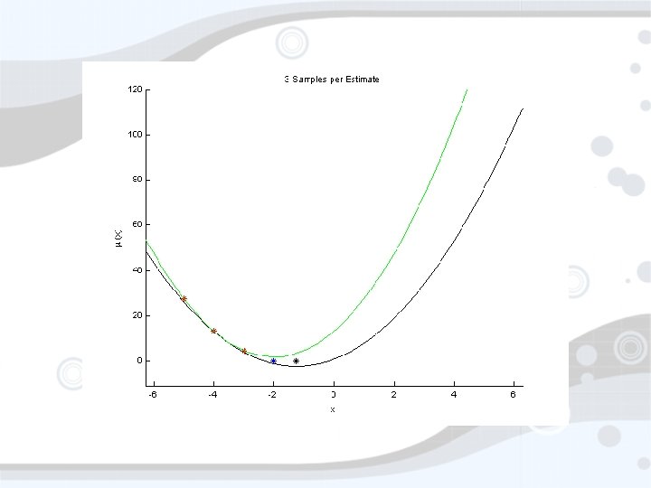
Does choice of x matter? • Clearly. • A frequentist would probably try to choose x to minimize the variance of -b/2 a • Can’t do that without knowing the real function • Some sort of sequential decision process…

Bayesian Approach • A Bayesian: • Has a prior • Gets data • Computes a posterior • In this case, prior and posterior over F • Encoding our uncertainty about F enables principled decision making • Everybody loves Gaussians

Gaussian • Unimodal • Concentrated • Easy to compute with • Sometimes • Tons of crazy properties

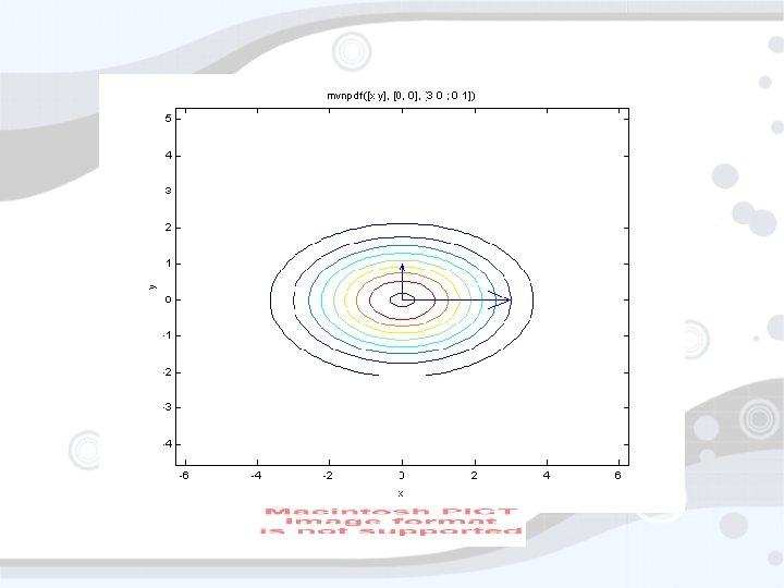
Multivariate Gaussian • Same thing, but moreso • Some things are harder • No nice form for cdf • Classical view: Points

Covariance Matrix • Shape param • Eigenstuff indicates variance and correlations

Higher Dimensions • Visualizing > 3 dimensions is…difficult • Thinking about vectors in the ‘i, j, k’ engineering sense is a trap • Means and marginals is practical • But then we don’t see correlations • Marginal distributions are Gaussian • ex. , F 6 ~ N(µ(F 6), σ(F 6)) σ(F 6) µ(F 6)

Yet Higher Dimensions • Why stop there? • We indexed before with ℤ. Why not ℝ? • Need functions µ(Fx), σ(Fx, Fy) for all x, y ∈ℝ • F is now an uncountably infinite dimensional vector • Don’t panic: It’s just a function

Getting Ridiculous • Why stop there? • We indexed before with ℝ. Why not ℝd? • Need functions µ(Fx), σ2(Fx, Fy) for all x, y ∈ℝd

Gaussian Process • Probability distribution indexed by an arbitrary set • Each element gets a Gaussian distribution over the reals with mean µ(x) • These distributions are dependent/correlated as defined by σ2(Fx, Fy) • Any subset of indices defines a multivariate gaussian distribution

Gaussian Process • Index set can be pretty much whatever • • • Reals Real vectors Graphs Strings … • Most interesting structure is in σ2(Fx, Fy), the ‘kernel. ’

Bayesian Updates for GPs • Oh yeah… Bayesian, remember? • How do Bayesians use a Gaussian Process? • Start with GP prior • Get some data • Compute a posterior • Ask interesting questions about the posterior

Prior

Data

Posterior

• Given Computing the Posterior • Prior • List of observed data points Fobs • (indexed by a list o 1, o 2, …, oj • List of query points Fask • (indexed by a list a 1, a 2, …, ak)

What now? • We constantly have a model Fpost of our function F • As we accumulate data, the model improves • How should we accumulate data? • Use the model to select which point to sample next

Candidate Selection • Caveat: This will take some work. • Only useful if F is expensive to evaluate • Dog walking is ~10 s �per evaluation • Here are some ideas�
 have the")
Idea 0: Min Posterior Mean • For which point x does F(x) have the lowest posterior mean? • This is, in general, a non-convex, global optimization problem. • WHAT? ? !! • I know, but remember F is expensive • Problems • Trapped in local minima (below prior mean) • Does not acknowledge model uncertainty

Idea 1: Thompson Sampling • Idea 0 is too dumb. • Sample a function from the posterior • Can only be sampled at a list of points • Minimize the sampled function • This returns a sample from P(X is min) • XT ~ P(F(X) < F(X’) forall X’) • Problems: • Explores too much

Idea 2: PMin • Thompson is more sensible, but still not quite right • Why not select • �� x = argmin P(F(X) < F(X’) forall X’) • i. e. , sample F(x) next where x is most likely to be the minimum of the function • Because it’s hard • Or at least I can’t do it. Our domain’s kinda big. • We can simulate this with repeated Thompson sampling • This is the optimal greedy action*

Finally… • AIBOS!

Seriously… • …did we have to go through all that to get to the dogs? • Yeah, sorry. • Now it’s easy: • An AIBO walk is a map from R 51 to R • 51 motion parameters map to velocity • Optimize the parameters to go fast

AIBO Walking • Set up a Gaussian process over R 51 • Kernel is also Gaussian (careful!) • Parameters for priors found by maximum likelihood • We could be more Bayesian here and use priors over the model parameters • Walk, get velocity, pick new parameters, walk

AIBO Walking • Results? • Pretty not too bad! • But not earth-shattering • Even choosing uniformly random parameters isn’t too bad • But using, say PMax shows a definite improvement • I think there’s more structure in the problem than people let on

Whew. • I need a break • Does anybody have any questions or brilliant ideas?
- Slides: 38