Econ 384 Intermediate Microeconomics II Instructor Lorne Priemaza

Econ 384 Intermediate Microeconomics II Instructor: Lorne Priemaza Lorne. priemaza@ualberta. ca

A. Intertemporal Choice A. 1 Compounding A. 2 Present Value A. 3 Present Value Decisions A. 4 Lifecycle Model

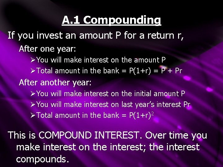
A. 1 Compounding If you invest an amount P for a return r, After one year: ØYou will make interest on the amount P ØTotal amount in the bank = P(1+r) = P + Pr After another year: ØYou will make interest on the initial amount P ØYou will make interest on last year’s interest Pr ØTotal amount in the bank = P(1+r)2 This is COMPOUND INTEREST. Over time you make interest on the interest; the interest compounds.

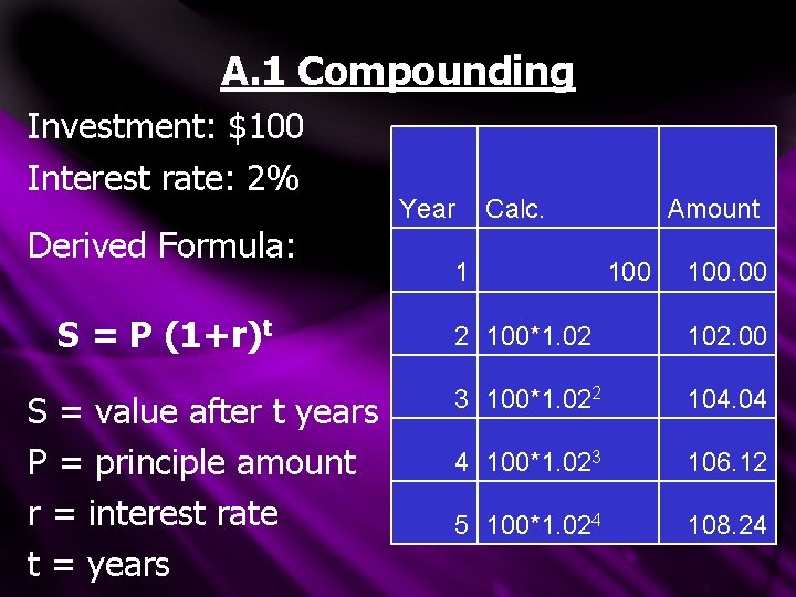
A. 1 Compounding Investment: $100 Interest rate: 2% Derived Formula: S = P (1+r)t S = value after t years P = principle amount r = interest rate t = years Year Calc. 1 Amount 100. 00 2 100*1. 02 102. 00 3 100*1. 022 104. 04 4 100*1. 023 106. 12 5 100*1. 024 108. 24

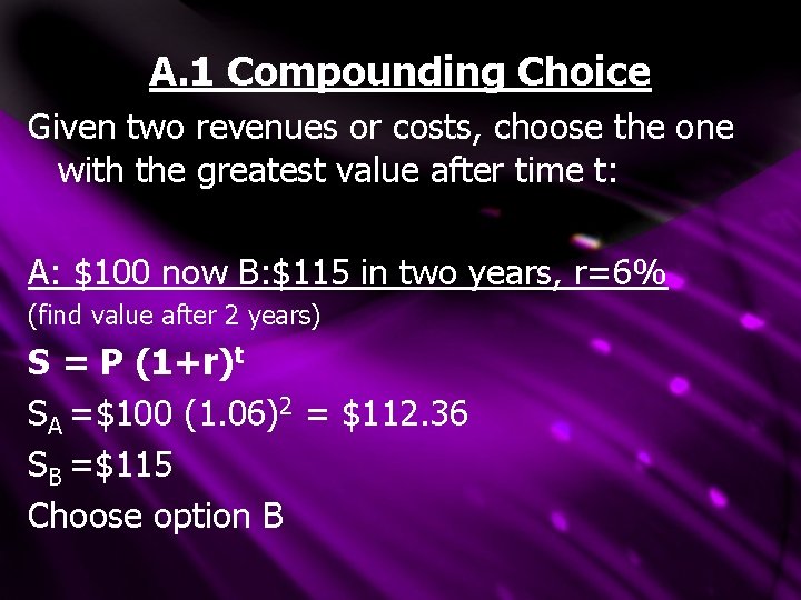
A. 1 Compounding Choice Given two revenues or costs, choose the one with the greatest value after time t: A: $100 now B: $115 in two years, r=6% (find value after 2 years) S = P (1+r)t SA =$100 (1. 06)2 = $112. 36 SB =$115 Choose option B

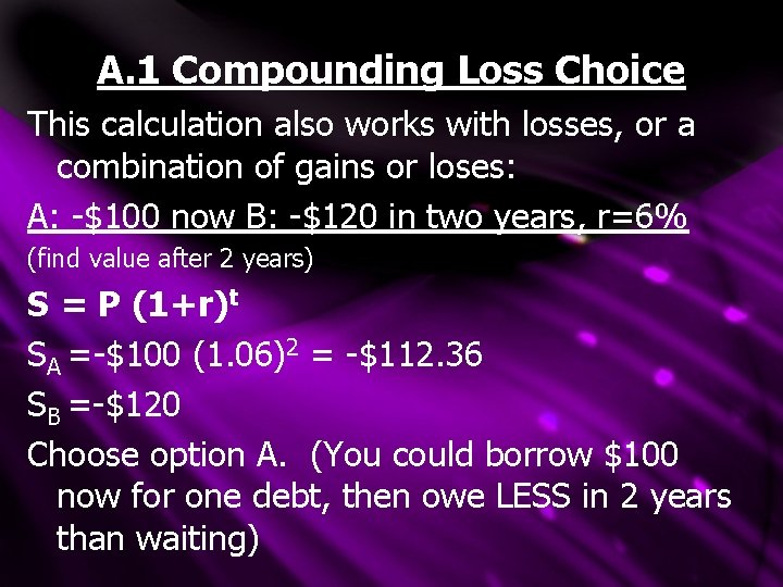
A. 1 Compounding Loss Choice This calculation also works with losses, or a combination of gains or loses: A: -$100 now B: -$120 in two years, r=6% (find value after 2 years) S = P (1+r)t SA =-$100 (1. 06)2 = -$112. 36 SB =-$120 Choose option A. (You could borrow $100 now for one debt, then owe LESS in 2 years than waiting)

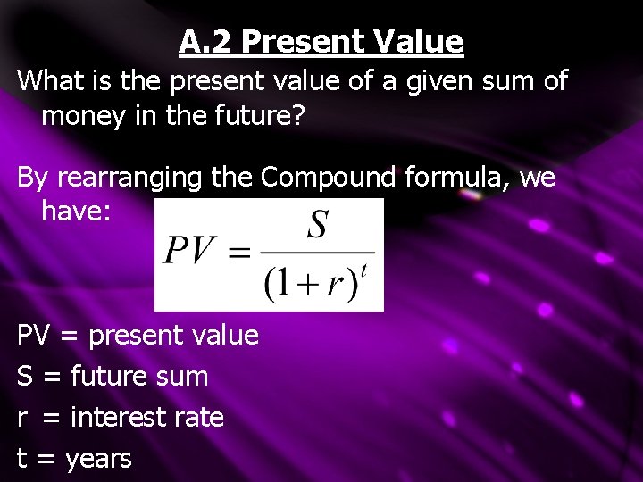
A. 2 Present Value What is the present value of a given sum of money in the future? By rearranging the Compound formula, we have: PV = present value S = future sum r = interest rate t = years

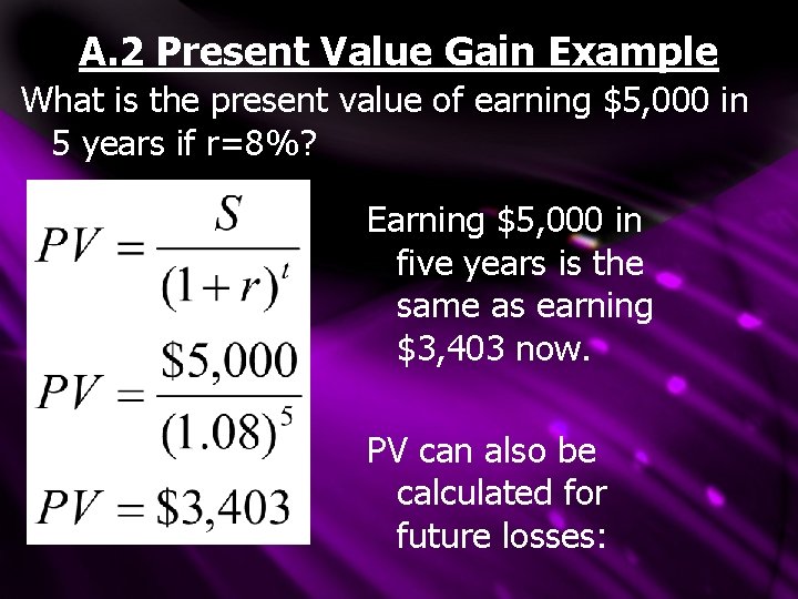
A. 2 Present Value Gain Example What is the present value of earning $5, 000 in 5 years if r=8%? Earning $5, 000 in five years is the same as earning $3, 403 now. PV can also be calculated for future losses:

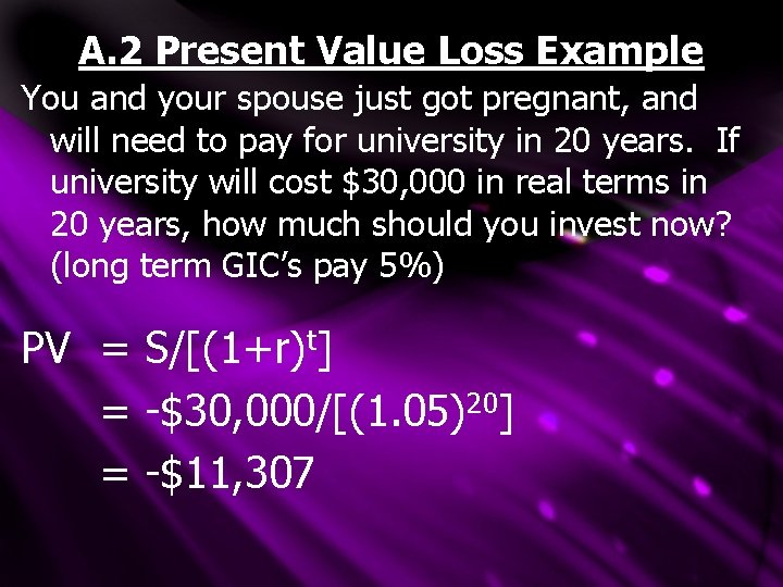
A. 2 Present Value Loss Example You and your spouse just got pregnant, and will need to pay for university in 20 years. If university will cost $30, 000 in real terms in 20 years, how much should you invest now? (long term GIC’s pay 5%) PV = S/[(1+r)t] = -$30, 000/[(1. 05)20] = -$11, 307

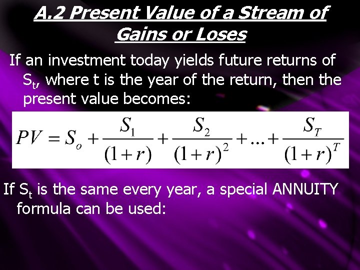
A. 2 Present Value of a Stream of Gains or Loses If an investment today yields future returns of St, where t is the year of the return, then the present value becomes: If St is the same every year, a special ANNUITY formula can be used:

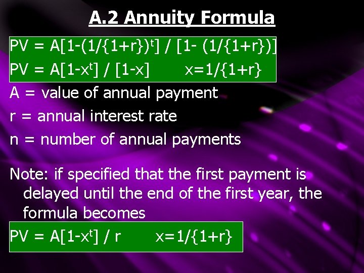
A. 2 Annuity Formula PV = A[1 -(1/{1+r})t] / [1 - (1/{1+r})] PV = A[1 -xt] / [1 -x] x=1/{1+r} A = value of annual payment r = annual interest rate n = number of annual payments Note: if specified that the first payment is delayed until the end of the first year, the formula becomes PV = A[1 -xt] / r x=1/{1+r}

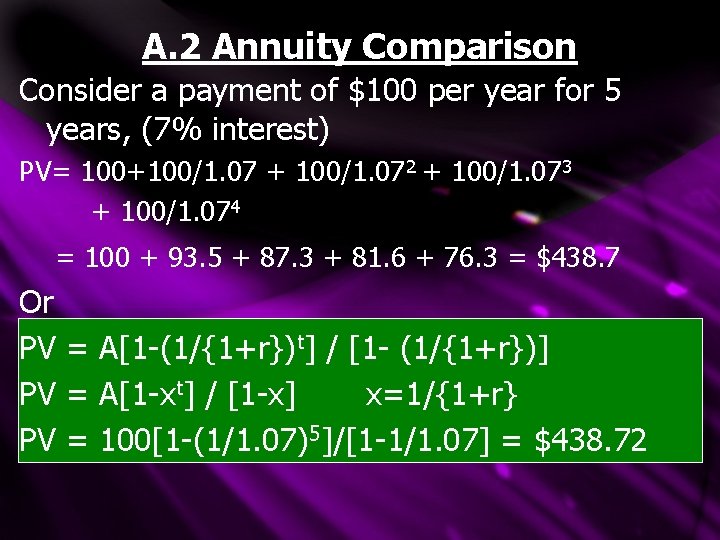
A. 2 Annuity Comparison Consider a payment of $100 per year for 5 years, (7% interest) PV= 100+100/1. 07 + 100/1. 072 + 100/1. 073 + 100/1. 074 = 100 + 93. 5 + 87. 3 + 81. 6 + 76. 3 = $438. 7 Or PV = A[1 -(1/{1+r})t] / [1 - (1/{1+r})] PV = A[1 -xt] / [1 -x] x=1/{1+r} PV = 100[1 -(1/1. 07)5]/[1 -1/1. 07] = $438. 72

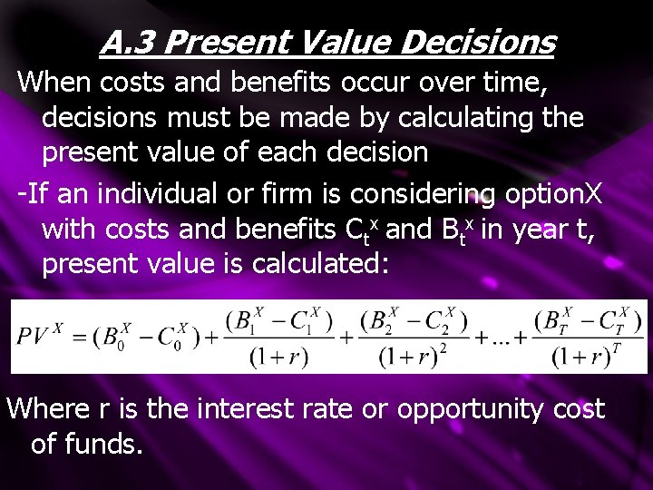
A. 3 Present Value Decisions When costs and benefits occur over time, decisions must be made by calculating the present value of each decision -If an individual or firm is considering option. X with costs and benefits Ctx and Btx in year t, present value is calculated: Where r is the interest rate or opportunity cost of funds.

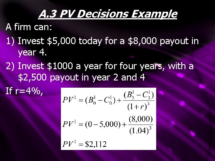
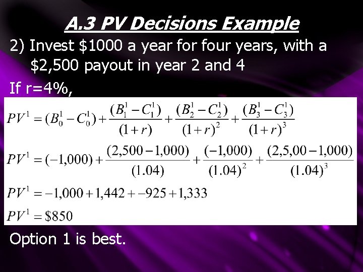
A. 3 PV Decisions Example A firm can: 1) Invest $5, 000 today for a $8, 000 payout in year 4. 2) Invest $1000 a year four years, with a $2, 500 payout in year 2 and 4 If r=4%,

A. 3 PV Decisions Example 2) Invest $1000 a year four years, with a $2, 500 payout in year 2 and 4 If r=4%, Option 1 is best.

A. 4 Lifecycle Model ØAlternately, often an individual needs to decide WHEN to consume over a lifetime ØTo examine this, one can sue a LIFECYCLE MODEL*: *Note: There alternate terms for the Lifecycle Model and the curves and calculations seen in this section

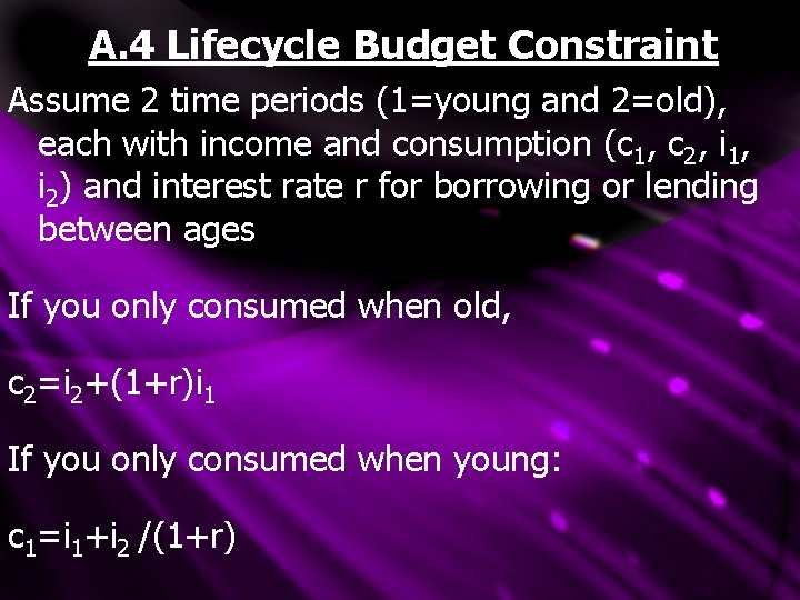
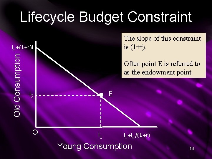
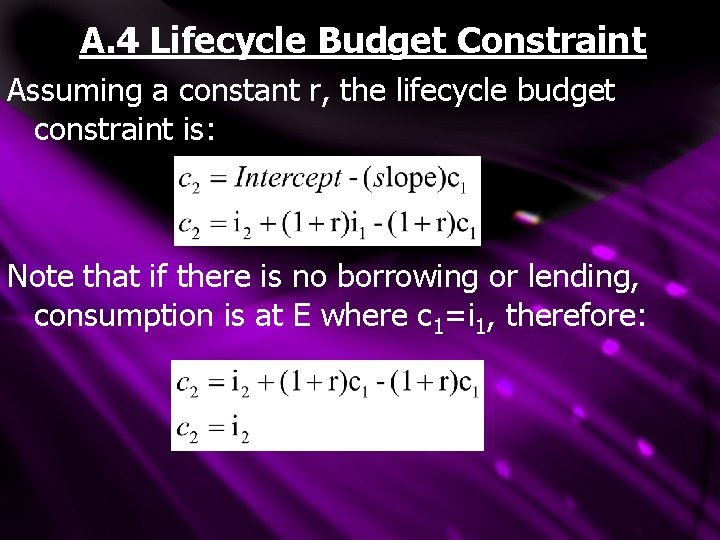
A. 4 Lifecycle Budget Constraint Assume 2 time periods (1=young and 2=old), each with income and consumption (c 1, c 2, i 1, i 2) and interest rate r for borrowing or lending between ages If you only consumed when old, c 2=i 2+(1+r)i 1 If you only consumed when young: c 1=i 1+i 2 /(1+r)

Lifecycle Budget Constraint The slope of this constraint is (1+r). Old Consumption i 2+(1+r)i 1 Often point E is referred to as the endowment point. i 2 O E i 1+i 2 /(1+r) Young Consumption 18

A. 4 Lifecycle Budget Constraint Assuming a constant r, the lifecycle budget constraint is: Note that if there is no borrowing or lending, consumption is at E where c 1=i 1, therefore:

A. 4 Lifetime Utility • In the lifecycle model, an individual’s lifetime utility is a function of the consumption in each time period: U=f(c 1, c 2) • If the consumer assumptions of consumer theory hold across time (completeness, transitivity, non-satiation) , this produces wellbehaved intertemporal indifference curves: 20

A. 4 Intertemporal Indifference Curves • Each INDIFFERENCE CURVE plots all the goods combinations that yield the same utility; that a person is indifferent between • These indifference curves have similar properties to typical consumer indifference curves (completeness, transitivity, negative slope, thin curves) 21

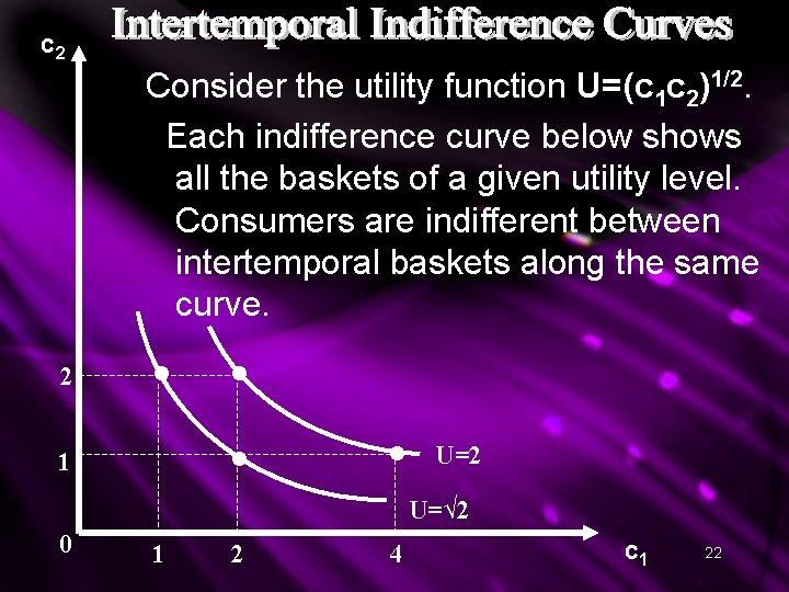
c 2 Consider the utility function U=(c 1 c 2)1/2. Each indifference curve below shows all the baskets of a given utility level. Consumers are indifferent between intertemporal baskets along the same curve. 2 • • • 1 • U=2 U=√ 2 0 1 2 4 c 1 22

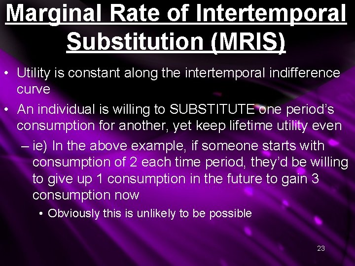
Marginal Rate of Intertemporal Substitution (MRIS) • Utility is constant along the intertemporal indifference curve • An individual is willing to SUBSTITUTE one period’s consumption for another, yet keep lifetime utility even – ie) In the above example, if someone starts with consumption of 2 each time period, they’d be willing to give up 1 consumption in the future to gain 3 consumption now • Obviously this is unlikely to be possible 23

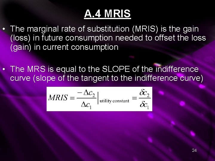
A. 4 MRIS • The marginal rate of substitution (MRIS) is the gain (loss) in future consumption needed to offset the loss (gain) in current consumption • The MRS is equal to the SLOPE of the indifference curve (slope of the tangent to the indifference curve) 24

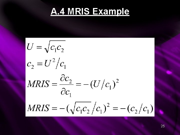
A. 4 MRIS Example 25

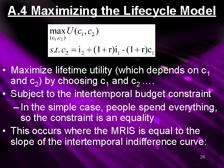
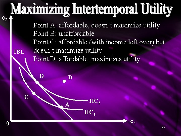
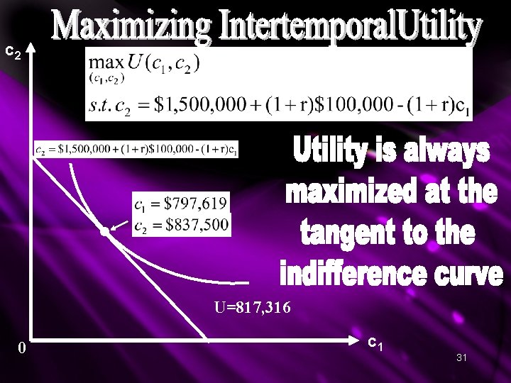
A. 4 Maximizing the Lifecycle Model • Maximize lifetime utility (which depends on c 1 and c 2) by choosing c 1 and c 2 …. • Subject to the intertemporal budget constraint – In the simple case, people spend everything, so the constraint is an equality • This occurs where the MRIS is equal to the slope of the intertemporal indifference curve: 26

c 2 IBL Point A: affordable, doesn’t maximize utility Point B: unaffordable Point C: affordable (with income left over) but doesn’t maximize utility Point D: affordable, maximizes utility • C • D • • 0 B A IIC 2 IIC 1 c 1 27

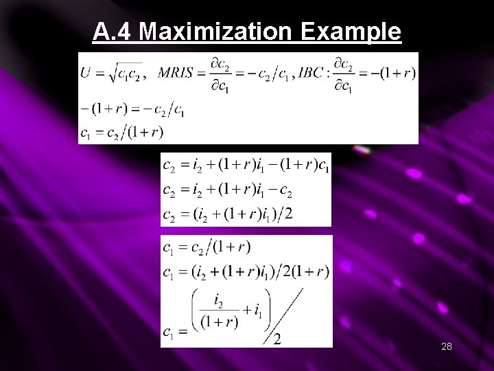
A. 4 Maximization Example 28

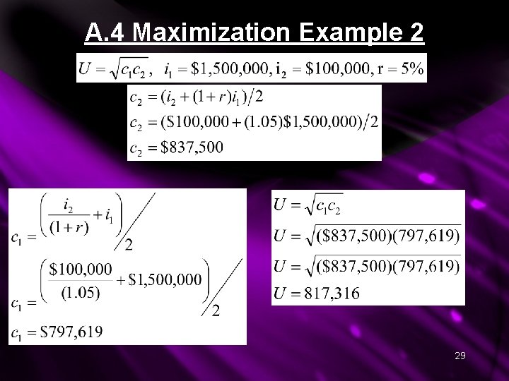
A. 4 Maximization Example 2 29

A. 4 Maximization Conclusion Lifetime utility is maximized at 817, 316 when $797, 619 is consumed when young and $837, 500 is consumed when old. *Always include a conclusion

c 2 • U=817, 316 0 c 1 31

A. Conclusion 1) Streams of intertemporal costs and benefits can be compared by comparing present values 2) To examine consumption timing, one can use the LIFECYCLE MODEL: a) An intertemporal budget line has a slope of (1+r) b) The slope of the intertemporal indifference curve is the Marginal Rate of Intertemporal Substitution (MRIS) c) Equating these allows us to Maximize 32