DMF model and exchange rate overshooting Lecture 1

DMF model and exchange rate overshooting Lecture 1, MSc Open Economy Macroeconomics, Birmingham, Autumn 2015 Tony Yates

Motivation • Dornbusch (1976) writing shortly after demise (1973) of fixed exchange rate system agreed at Bretton Woods • Era of exchange rate volatility [that continued of course]; fluctuations seemed to exceed what was sensible from fundamentals • ‘Overshooting’ provided the answer.

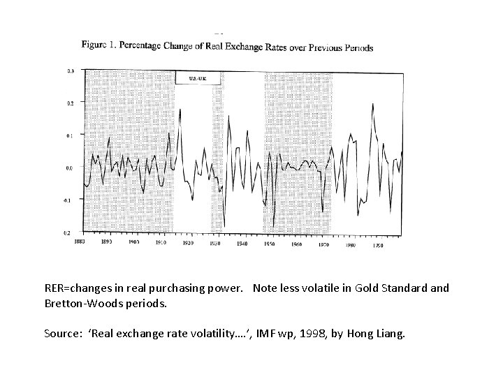
RER=changes in real purchasing power. Note less volatile in Gold Standard and Bretton-Woods periods. Source: ‘Real exchange rate volatility…. ’, IMF wp, 1998, by Hong Liang.

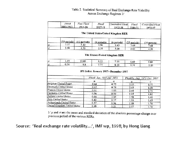
Source: ‘Real exchange rate volatility…. ’, IMF wp, 1998, by Hong Liang

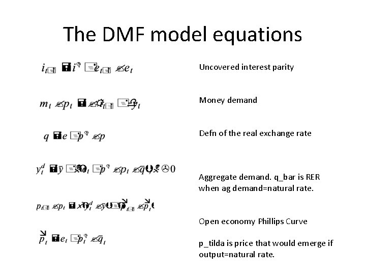
The DMF model equations Uncovered interest parity Money demand Defn of the real exchange rate Aggregate demand. q_bar is RER when ag demand=natural rate. Open economy Phillips Curve p_tilda is price that would emerge if output=natural rate.

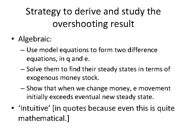
Strategy to derive and study the overshooting result • Algebraic: – Use model equations to form two difference equations, in q and e. – Solve them to find their steady states in terms of exogenous money stock. – Show that when we change money, e movement initially exceeds eventual new steady state. • ‘Intuitive’ [in quotes because even this is quite mathematical. ]

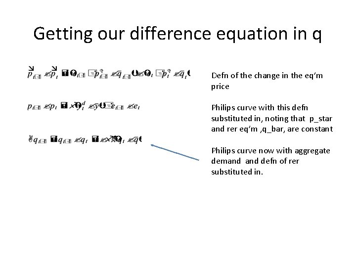
Getting our difference equation in q Defn of the change in the eq’m price Philips curve with this defn substituted in, noting that p_star and rer eq’m , q_bar, are constant Philips curve now with aggregate demand defn of rer substituted in.

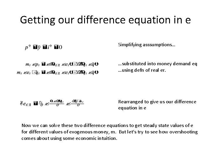
Getting our difference equation in e Simplifying asssumptions… …substituted into money demand eq …using defn of real er. Rearranged to give us our difference equation in e Now we can solve these two difference equations to get steady state values of e for different values of exogenous money, m. But let’s try to see how overshooting comes about using some economic intuition.

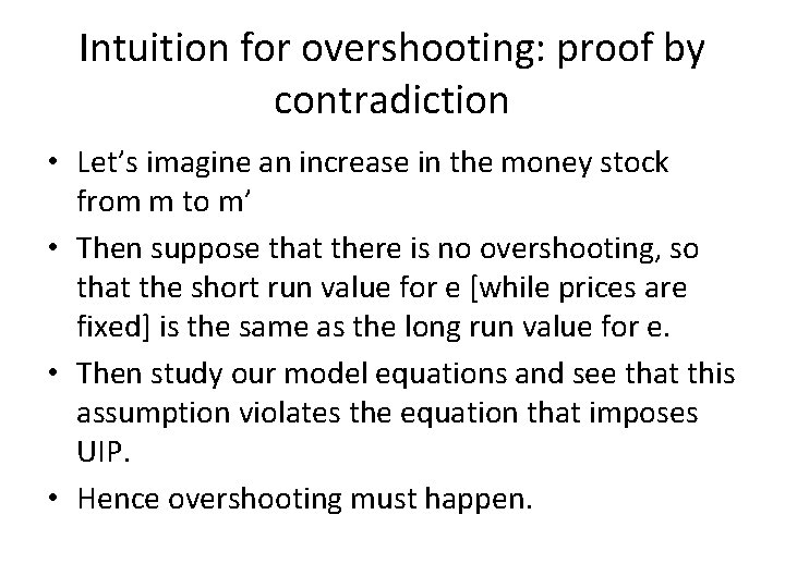
Intuition for overshooting: proof by contradiction • Let’s imagine an increase in the money stock from m to m’ • Then suppose that there is no overshooting, so that the short run value for e [while prices are fixed] is the same as the long run value for e. • Then study our model equations and see that this assumption violates the equation that imposes UIP. • Hence overshooting must happen.

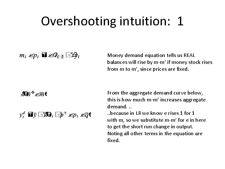
Overshooting intuition: 1 Money demand equation tells us REAL balances will rise by m-m’ if money stock rises from m to m’, since prices are fixed. From the aggregate demand curve below, this is how much m-m’ increases aggregate demand. . . because in LR we know e rises 1 for 1 with m, so we substitute m-m’ for e in here to get the short run change in output. Noting all other terms in the equation are fixed.

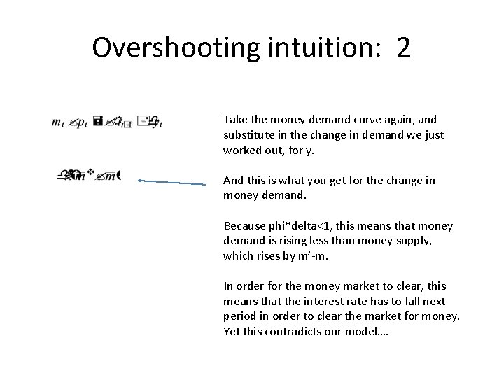
Overshooting intuition: 2 Take the money demand curve again, and substitute in the change in demand we just worked out, for y. And this is what you get for the change in money demand. Because phi*delta<1, this means that money demand is rising less than money supply, which rises by m’-m. In order for the money market to clear, this means that the interest rate has to fall next period in order to clear the market for money. Yet this contradicts our model….

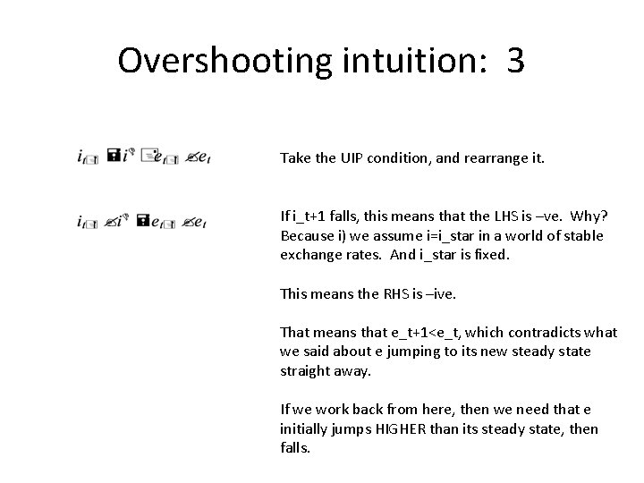
Overshooting intuition: 3 Take the UIP condition, and rearrange it. If i_t+1 falls, this means that the LHS is –ve. Why? Because i) we assume i=i_star in a world of stable exchange rates. And i_star is fixed. This means the RHS is –ive. That means that e_t+1<e_t, which contradicts what we said about e jumping to its new steady state straight away. If we work back from here, then we need that e initially jumps HIGHER than its steady state, then falls.

Assumptions required to get overshooting • Phi*delta<1 [? ] • Prices sticky for one period [ok] • Perfect foresight rational expectations [in fin mkts, maybe, but prob not] • Particular conjectured functional forms for money demand [this one ok], aggregate demand [contestable], Phillips Curve [likewise]. • No microfoundations to assess whether these are possible worlds. • Empirically controversial model components.

Word on next lecture • Controversial model with clear hypothesis: money supply changes cause volatility in e. • We will look at time series VAR techniques for testing this and related models. • Relies on deducing monetary shocks from long run neutrality in how they affect real things. • Then measuring contribution of monetary shocks to everything.

Deriving overshooting analytically • Solve our two difference equations, essentially by repeated forward substitution. • Substitute the solution for q into the solution for e, which will be in terms of m. • Then study dynamics of e in response to change from m to m’, and prove conditions under which e overshoots.

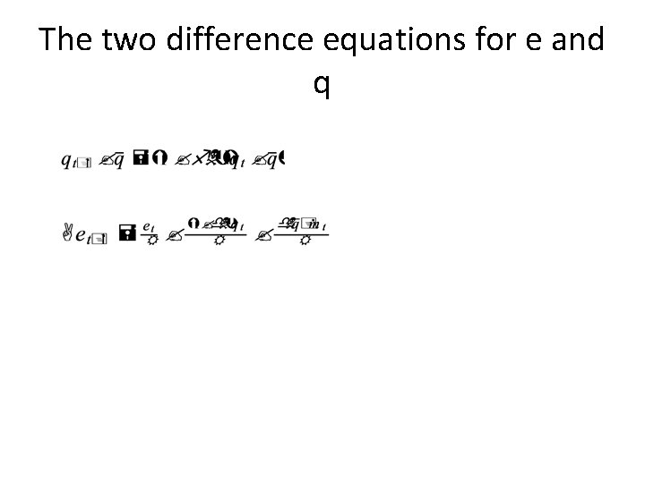
The two difference equations for e and q

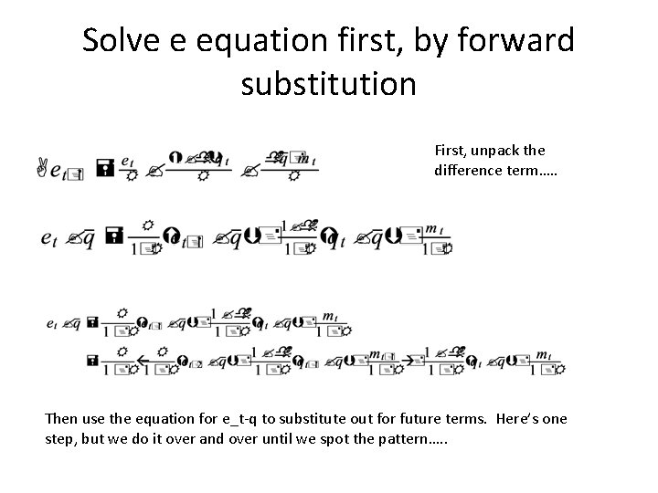
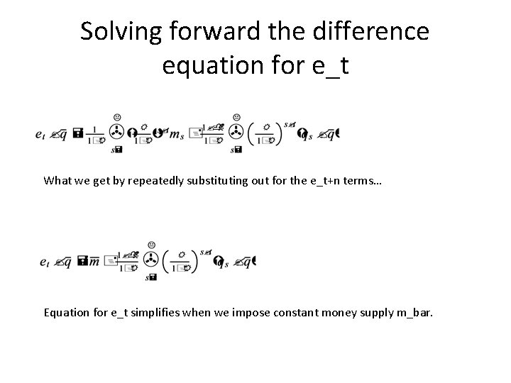
Solve e equation first, by forward substitution First, unpack the difference term…. . Then use the equation for e_t-q to substitute out for future terms. Here’s one step, but we do it over and over until we spot the pattern…. .

Solving forward the difference equation for e_t What we get by repeatedly substituting out for the e_t+n terms… Equation for e_t simplifies when we impose constant money supply m_bar.

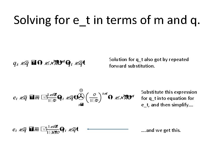
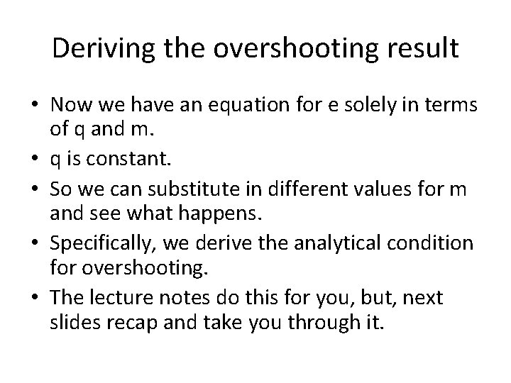
Solving for e_t in terms of m and q. Solution for q_t also got by repeated forward substitution. Substitute this expression for q_t into equation for e_t, and then simplify…. …. and we get this.

Deriving the overshooting result • Now we have an equation for e solely in terms of q and m. • q is constant. • So we can substitute in different values for m and see what happens. • Specifically, we derive the analytical condition for overshooting. • The lecture notes do this for you, but, next slides recap and take you through it.

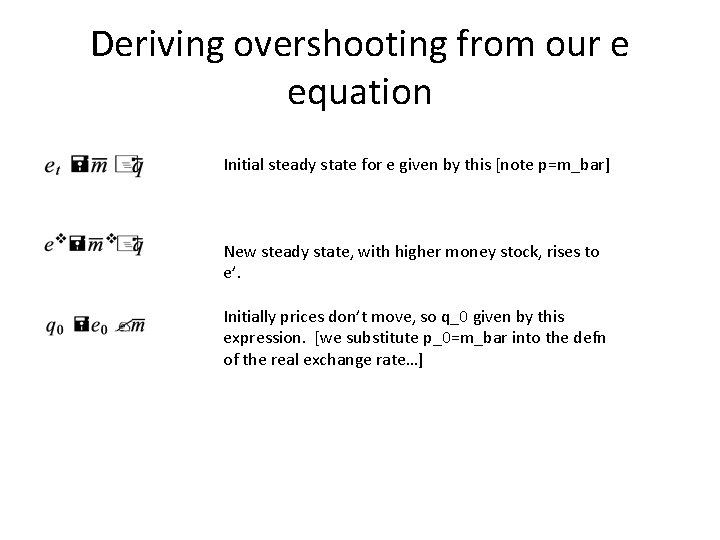
Deriving overshooting from our e equation Initial steady state for e given by this [note p=m_bar] New steady state, with higher money stock, rises to e’. Initially prices don’t move, so q_0 given by this expression. [we substitute p_0=m_bar into the defn of the real exchange rate…]

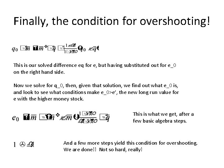
Finally, the condition for overshooting! This is our solved difference eq for e, but having substituted out for e_0 on the right hand side. Now we solve for q_0, then, given that solution, we find out what e_0 is, and look to see what conditions make e_0>e’, the new long run value for e with the higher money stock. This is what we get, after a few basic algebra steps. And a few more steps yield this condition for overshooting. We are done!! Not so hard, really!

Recap • DMF model consisted of: – Money demand relation – Open economy Phillips Curve – Aggregate demand equation – Assumption of perfect foresight RE

Two strategies for deriving the overshooting result • First was to prove by contradiction – We supposed that the short and long run e were the same after an increase of m to m’ – And we realised this contradicted the UIP condition • Second was to solve algebraically, forming difference equations in e and q, solving them forward by repeated substitution.

Overshooting: so what? Why do we care? • DMF provided a rational for exchange rate volatility seen in floating ex rate regimes. • Suggests a route whereby we can get significant welfare costs from unwarranted monetary policy shocks. • Shows the strengths and weaknesses of oldstyle macroeconomic RE modelling. • S: powerful results. W: where do these curves come from?

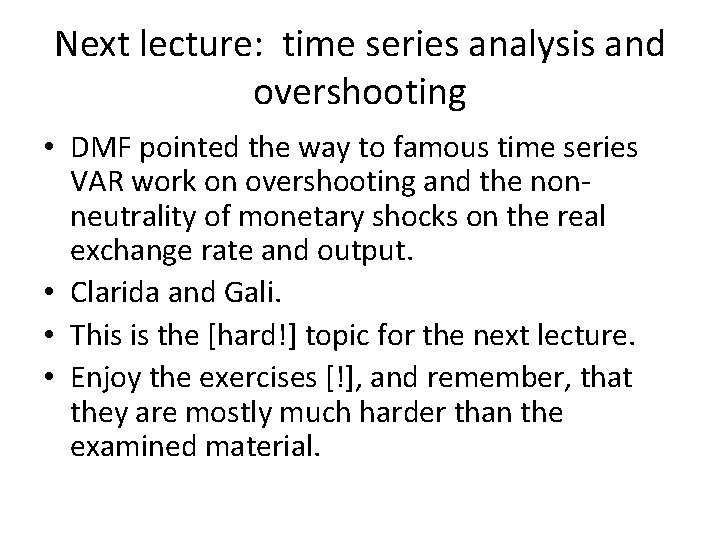
Next lecture: time series analysis and overshooting • DMF pointed the way to famous time series VAR work on overshooting and the nonneutrality of monetary shocks on the real exchange rate and output. • Clarida and Gali. • This is the [hard!] topic for the next lecture. • Enjoy the exercises [!], and remember, that they are mostly much harder than the examined material.