Disjoint Sets Data Structure Chap 21 A disjointset

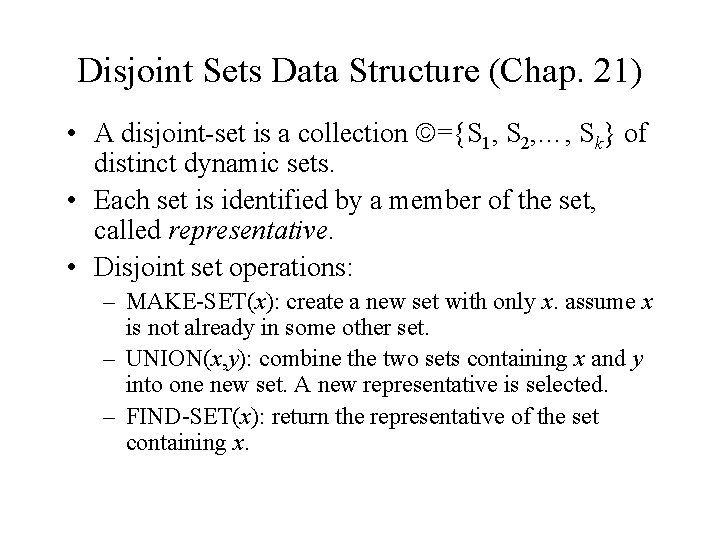
Disjoint Sets Data Structure (Chap. 21) • A disjoint-set is a collection ={S 1, S 2, …, Sk} of distinct dynamic sets. • Each set is identified by a member of the set, called representative. • Disjoint set operations: – MAKE-SET(x): create a new set with only x. assume x is not already in some other set. – UNION(x, y): combine the two sets containing x and y into one new set. A new representative is selected. – FIND-SET(x): return the representative of the set containing x.

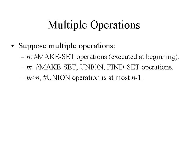
Multiple Operations • Suppose multiple operations: – n: #MAKE-SET operations (executed at beginning). – m: #MAKE-SET, UNION, FIND-SET operations. – m n, #UNION operation is at most n-1.

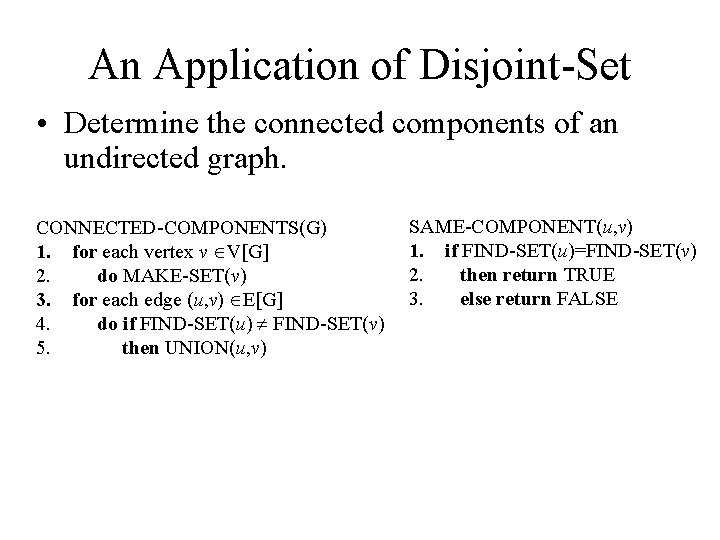
An Application of Disjoint-Set • Determine the connected components of an undirected graph. CONNECTED-COMPONENTS(G) 1. for each vertex v V[G] 2. do MAKE-SET(v) 3. for each edge (u, v) E[G] 4. do if FIND-SET(u) FIND-SET(v) 5. then UNION(u, v) SAME-COMPONENT(u, v) 1. if FIND-SET(u)=FIND-SET(v) 2. then return TRUE 3. else return FALSE

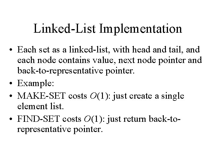
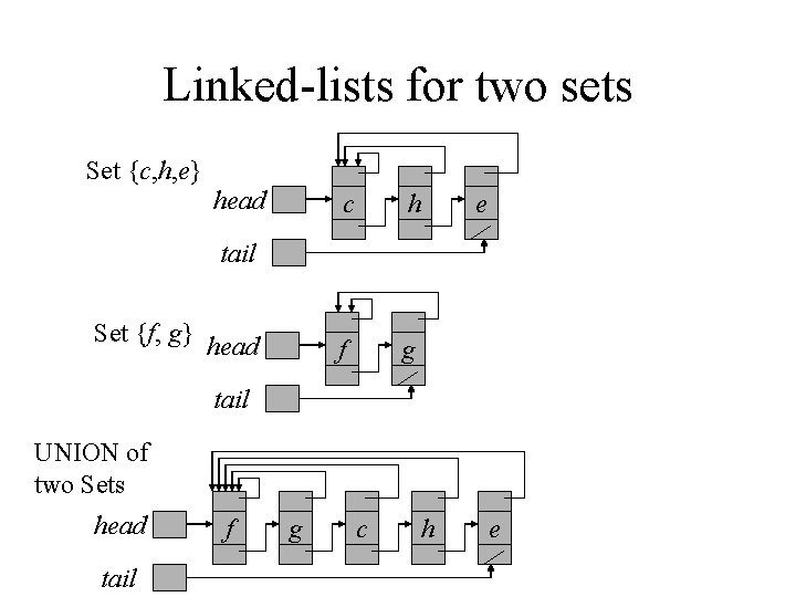
Linked-List Implementation • Each set as a linked-list, with head and tail, and each node contains value, next node pointer and back-to-representative pointer. • Example: • MAKE-SET costs O(1): just create a single element list. • FIND-SET costs O(1): just return back-torepresentative pointer.

Linked-lists for two sets Set {c, h, e} head c h f g e tail Set {f, g} head tail UNION of two Sets head tail f g c h e

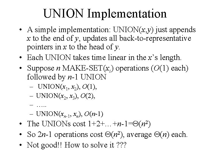
UNION Implementation • A simplementation: UNION(x, y) just appends x to the end of y, updates all back-to-representative pointers in x to the head of y. • Each UNION takes time linear in the x’s length. • Suppose n MAKE-SET(xi) operations (O(1) each) followed by n-1 UNION – – UNION(x 1, x 2), O(1), UNION(x 2, x 3), O(2), …. . UNION(xn-1, xn), O(n-1) • The UNIONs cost 1+2+…+n-1= (n 2) • So 2 n-1 operations cost (n 2), average (n) each. • Not good!! How to solve it ? ? ?

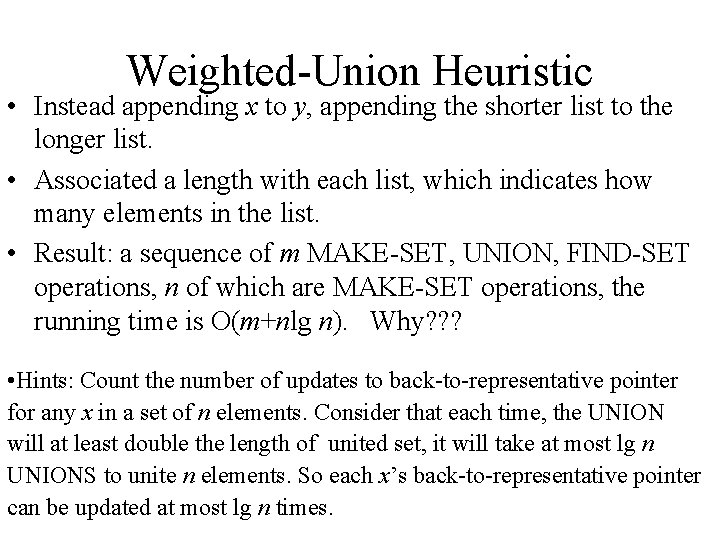
Weighted-Union Heuristic • Instead appending x to y, appending the shorter list to the longer list. • Associated a length with each list, which indicates how many elements in the list. • Result: a sequence of m MAKE-SET, UNION, FIND-SET operations, n of which are MAKE-SET operations, the running time is O(m+nlg n). Why? ? ? • Hints: Count the number of updates to back-to-representative pointer for any x in a set of n elements. Consider that each time, the UNION will at least double the length of united set, it will take at most lg n UNIONS to unite n elements. So each x’s back-to-representative pointer can be updated at most lg n times.

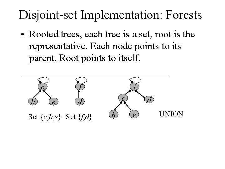
Disjoint-set Implementation: Forests • Rooted trees, each tree is a set, root is the representative. Each node points to its parent. Root points to itself. cf c h e cf c d Set {c, h, e} Set {f, d} h d e UNION

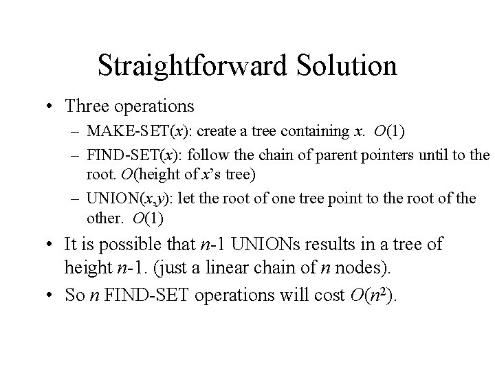
Straightforward Solution • Three operations – MAKE-SET(x): create a tree containing x. O(1) – FIND-SET(x): follow the chain of parent pointers until to the root. O(height of x’s tree) – UNION(x, y): let the root of one tree point to the root of the other. O(1) • It is possible that n-1 UNIONs results in a tree of height n-1. (just a linear chain of n nodes). • So n FIND-SET operations will cost O(n 2).

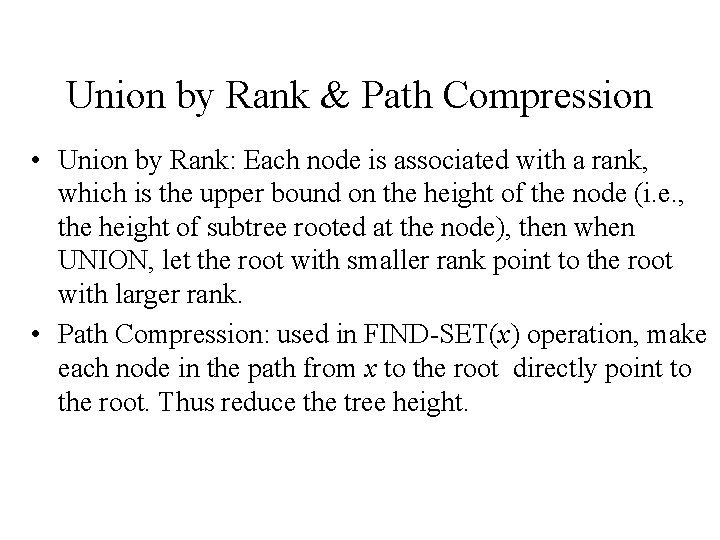
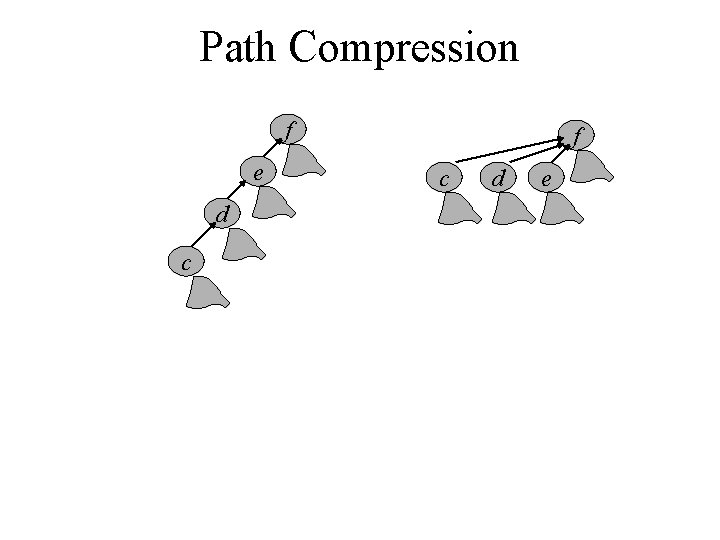
Union by Rank & Path Compression • Union by Rank: Each node is associated with a rank, which is the upper bound on the height of the node (i. e. , the height of subtree rooted at the node), then when UNION, let the root with smaller rank point to the root with larger rank. • Path Compression: used in FIND-SET(x) operation, make each node in the path from x to the root directly point to the root. Thus reduce the tree height.

Path Compression f e d c f c d e

Algorithm for Disjoint-Set Forest UNION(x, y) 1. LINK(FIND-SET(x), FIND-SET(y)) MAKE-SET(x) 1. p[x] x 2. rank[x] 0 LINK(x, y) 1. if rank[x]>rank[y] 2. then p[y] x 3. else p[x] y 4. if rank[x]=rank[y] 5. then rank[y]++ FIND-SET(x) 1. if x p[x] 2. then p[x] FIND-SET(p[x]) 3. return p[x] Worst case running time for m MAKE-SET, UNION, FIND-SET operations is: O(m (n)) where (n) 4. So nearly linear in m.

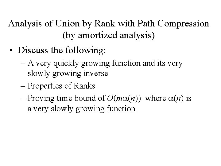
Analysis of Union by Rank with Path Compression (by amortized analysis) • Discuss the following: – A very quickly growing function and its very slowly growing inverse – Properties of Ranks – Proving time bound of O(m (n)) where (n) is a very slowly growing function.

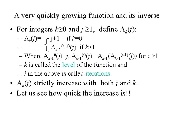
A very quickly growing function and its inverse • For integers k 0 and j 1, define Ak(j): – Ak(j)= j+1 if k=0 – Ak-1(j+1)(j) if k 1 – Where Ak-10(j)=j, Ak-1(i)(j)= Ak-1(i-1)(j)) for i 1. – k is called the level of the function and – i in the above is called iterations. • Ak(j) strictly increase with both j and k. • Let us see how quick the increase is!!

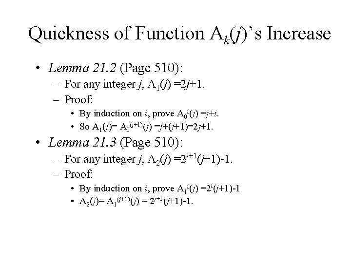
Quickness of Function Ak(j)’s Increase • Lemma 21. 2 (Page 510): – For any integer j, A 1(j) =2 j+1. – Proof: • By induction on i, prove A 0 i(j) =j+i. • So A 1(j)= A 0(j+1)(j) =j+(j+1)=2 j+1. • Lemma 21. 3 (Page 510): – For any integer j, A 2(j) =2 j+1(j+1)-1. – Proof: • By induction on i, prove A 1 i(j) =2 i(j+1)-1 • A 2(j)= A 1(j+1)(j) = 2 j+1(j+1)-1.

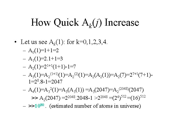
How Quick Ak(j) Increase • Let us see Ak(1): for k=0, 1, 2, 3, 4. – – A 0(1)=1+1=2 A 1(1)=2. 1+1=3 A 2(1)=21+1(1+1)-1=7 A 3(1)=A 2(1+1)(1)=A 2(2)(1)=A 2(1))=A 2(7)=27+1(7+1)1=28. 8 -1=2047 – A 4(1)=A 32(1)=A 3(1)) =A 3(2047)=A 2(2048)(2047) >> A 2(2047) =22048 -1 >22048 =(24)512 =(16)512 – >>1080. (estimated number of atoms in universe)

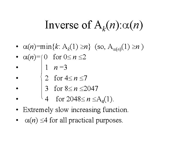
Inverse of Ak(n): (n) • • (n)=min{k: Ak(1) n} (so, A (n)(1) n ) (n)= 0 for 0 n 2 1 n =3 2 for 4 n 7 3 for 8 n 2047 4 for 2048 n A 4(1). Extremely slow increasing function. (n) 4 for all practical purposes.

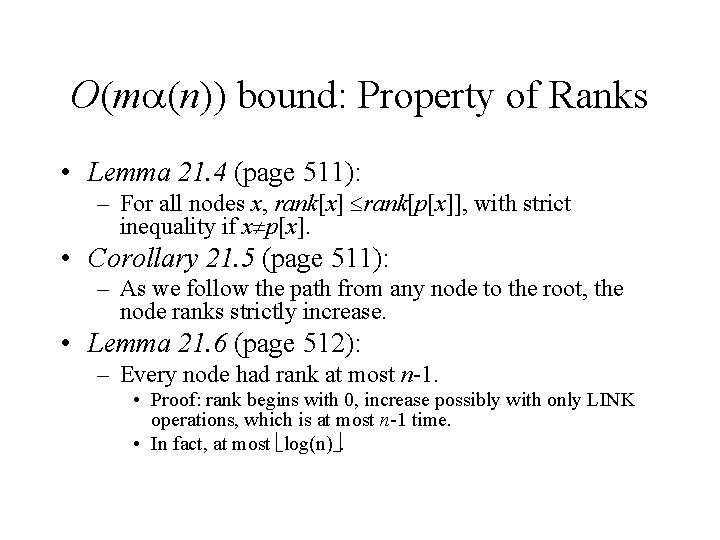
O(m (n)) bound: Property of Ranks • Lemma 21. 4 (page 511): – For all nodes x, rank[x] rank[p[x]], with strict inequality if x p[x]. • Corollary 21. 5 (page 511): – As we follow the path from any node to the root, the node ranks strictly increase. • Lemma 21. 6 (page 512): – Every node had rank at most n-1. • Proof: rank begins with 0, increase possibly with only LINK operations, which is at most n-1 time. • In fact, at most log(n).

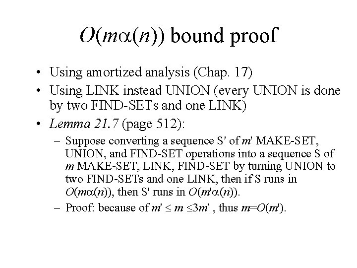
O(m (n)) bound proof • Using amortized analysis (Chap. 17) • Using LINK instead UNION (every UNION is done by two FIND-SETs and one LINK) • Lemma 21. 7 (page 512): – Suppose converting a sequence S' of m' MAKE-SET, UNION, and FIND-SET operations into a sequence S of m MAKE-SET, LINK, FIND-SET by turning UNION to two FIND-SETs and one LINK, then if S runs in O(m (n)), then S' runs in O(m' (n)). – Proof: because of m' m 3 m' , thus m=O(m').

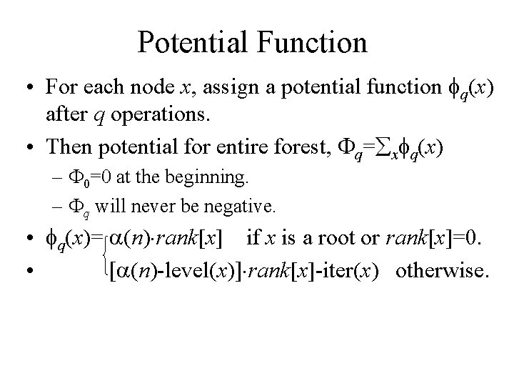
Potential Function • For each node x, assign a potential function q(x) after q operations. • Then potential for entire forest, q= x q(x) – 0=0 at the beginning. – q will never be negative. • q(x)= (n) rank[x] if x is a root or rank[x]=0. • (n)-level(x) rank[x]-iter(x) otherwise.

level(x) and iter(x) • level(x)=max{k: rank[p[x]] Ak(rank[x])} – 0 Level(x)< (n), since • rank[p[x]] rank[x]+1=A 0(rank[x]) and • A (n) (rank[x]) A (n) (1) n > rank[p[x]]. • iter(x)=max{i: rank[p[x]] Alevel(x)(i)(rank[x])} – 1 iter(x) rank[x], since • rank[p[x]] Alevel(x)(rank[x])=Alevel(x)(1)(rank[x]) and • Alevel(x)(rank[x]+1)(rank[x])=Alevel(x)+1(rank[x])>rank[p[x]].

Relations among rank[p[x]], level(x) and iter(x) • Since rank[p[x]] monotonically increase over time, in order for iter(x) to decrease, level(x) must increase. • Or say another way, as long as level(x) remains unchanged, iter(x) must either increase or remains unchanged.

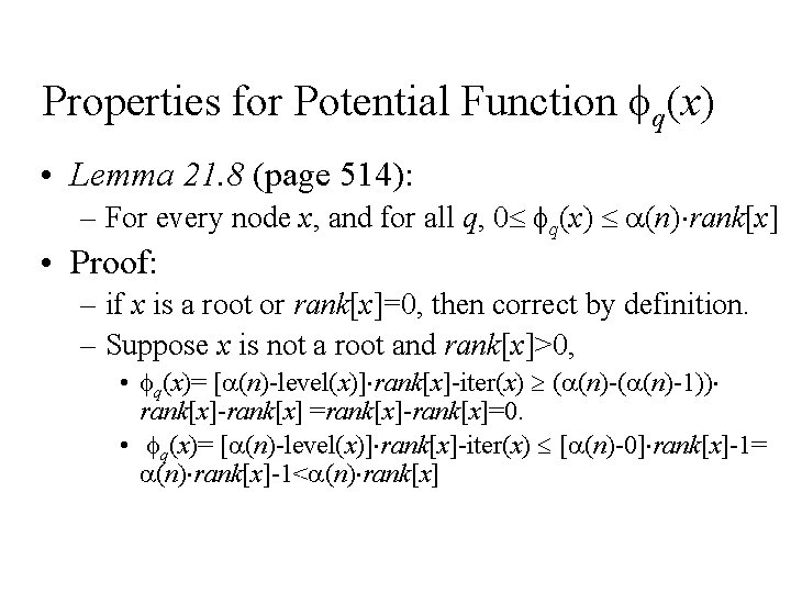
Properties for Potential Function q(x) • Lemma 21. 8 (page 514): – For every node x, and for all q, 0 q(x) (n) rank[x] • Proof: – if x is a root or rank[x]=0, then correct by definition. – Suppose x is not a root and rank[x]>0, • q(x)= [ (n)-level(x)] rank[x]-iter(x) ( (n)-1)) rank[x]-rank[x] =rank[x]-rank[x]=0. • q(x)= [ (n)-level(x)] rank[x]-iter(x) [ (n)-0] rank[x]-1= (n) rank[x]-1< (n) rank[x]

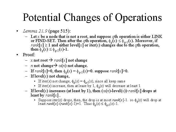
Potential Changes of Operations • Lemma 21. 9 (page 515): – Let x be a node that is not a root, and suppose qth operation is either LINK or FIND-SET. Then after the qth operation, q(x) q-1(x). Moreover, if rank[x] 1 and either level[x] or iter(x) changes due to the qth operation, then q(x) q-1(x)-1. • Proof: – – x not root rank[x] not change n not change (n) not change. If rank[x]=0, then q(x) = q-1(x)=0. suppose rank[x]>0. If level(x) not change, • If iter(x) not change, q(x) = q-1(x), since all keep same • If iter(x) increase, then at lease by 1, q(x) will decrease at least 1. – If level(x) increases (at least by 1), then ( (n)-level(x)) rank[x] drops at least by rank[x]. • Suppose iter(x) drops, then, the drop is at most rank[x]-1. so q(x) will drop at least rank[x]-(rank[x]-1)=1. Thus q(x) q-1(x)-1.

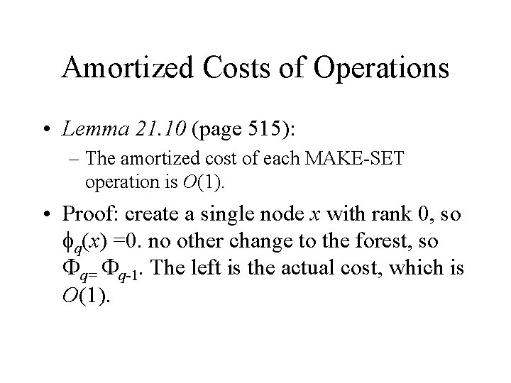
Amortized Costs of Operations • Lemma 21. 10 (page 515): – The amortized cost of each MAKE-SET operation is O(1). • Proof: create a single node x with rank 0, so q(x) =0. no other change to the forest, so q= q-1. The left is the actual cost, which is O(1).

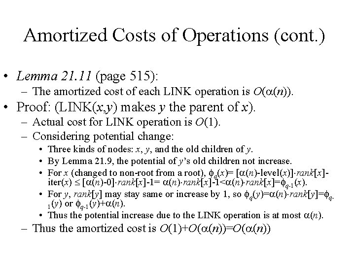
Amortized Costs of Operations (cont. ) • Lemma 21. 11 (page 515): – The amortized cost of each LINK operation is O( (n)). • Proof: (LINK(x, y) makes y the parent of x). – Actual cost for LINK operation is O(1). – Considering potential change: • Three kinds of nodes: x, y, and the old children of y. • By Lemma 21. 9, the potential of y’s old children not increase. • For x (changed to non-root from a root), q(x)= [ (n)-level(x)] rank[x]iter(x) [ (n)-0] rank[x]-1= (n) rank[x]-1< (n) rank[x]= q-1(x). • For y, rank[y] may stay same or increase by 1, so q(y)= (n) rank[y]= q 1(y) or q-1(y)+ (n). • Thus the potential increase due to the LINK operation is at most (n). – Thus the amortized cost is O(1)+O( (n))=O( (n))

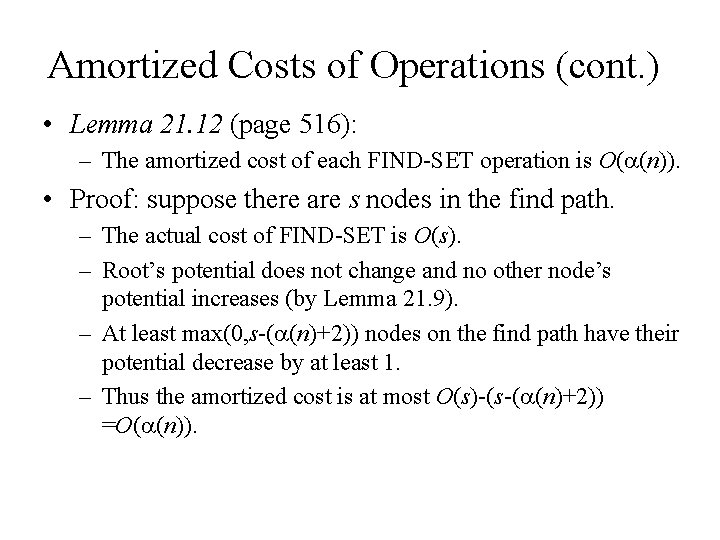
Amortized Costs of Operations (cont. ) • Lemma 21. 12 (page 516): – The amortized cost of each FIND-SET operation is O( (n)). • Proof: suppose there are s nodes in the find path. – The actual cost of FIND-SET is O(s). – Root’s potential does not change and no other node’s potential increases (by Lemma 21. 9). – At least max(0, s-( (n)+2)) nodes on the find path have their potential decrease by at least 1. – Thus the amortized cost is at most O(s)-(s-( (n)+2)) =O( (n)).

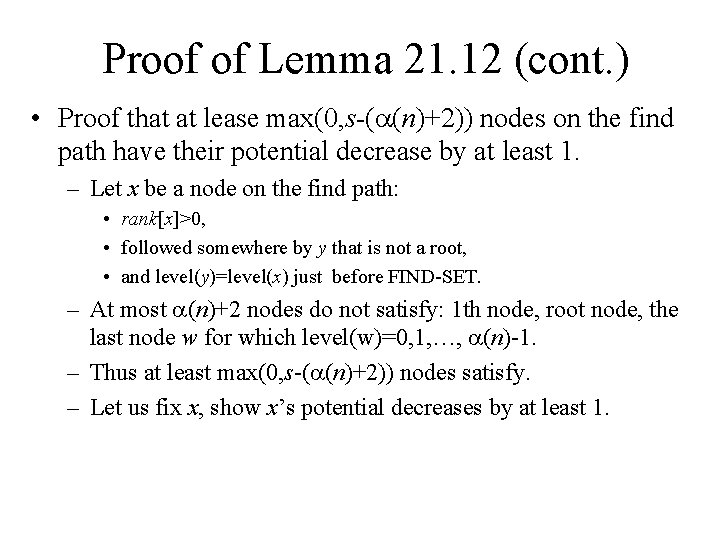
Proof of Lemma 21. 12 (cont. ) • Proof that at lease max(0, s-( (n)+2)) nodes on the find path have their potential decrease by at least 1. – Let x be a node on the find path: • rank[x]>0, • followed somewhere by y that is not a root, • and level(y)=level(x) just before FIND-SET. – At most (n)+2 nodes do not satisfy: 1 th node, root node, the last node w for which level(w)=0, 1, …, (n)-1. – Thus at least max(0, s-( (n)+2)) nodes satisfy. – Let us fix x, show x’s potential decreases by at least 1.

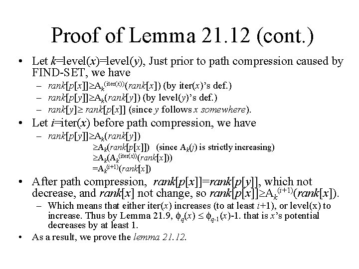
Proof of Lemma 21. 12 (cont. ) • Let k=level(x)=level(y), Just prior to path compression caused by FIND-SET, we have – rank[p[x]] Ak(iter(x))(rank[x]) (by iter(x)’s def. ) – rank[p[y]] Ak(rank[y]) (by level(y)’s def. ) – rank[y] rank[p[x]] (since y follows x somewhere). • Let i=iter(x) before path compression, we have – rank[p[y]] Ak(rank[y]) Ak(rank[p[x]]) (since Ak(j) is strictly increasing) Ak(Ak(iter(x))(rank[x])) =Ak(i+1)(rank[x]) • After path compression, rank[p[x]]=rank[p[y]], which not decrease, and rank[x] not change, so rank[p[x]] Ak(i+1)(rank[x]). – Which means that either iter(x) increases (to at least i+1), or level(x) to increase. Thus by Lemma 21. 9, q(x) q-1(x)-1. that is x’s potential decreases by at least 1. • As a result, we prove the lemma 21. 12.

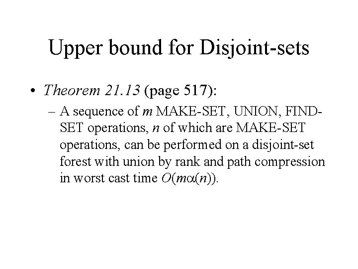
Upper bound for Disjoint-sets • Theorem 21. 13 (page 517): – A sequence of m MAKE-SET, UNION, FINDSET operations, n of which are MAKE-SET operations, can be performed on a disjoint-set forest with union by rank and path compression in worst cast time O(m (n)).

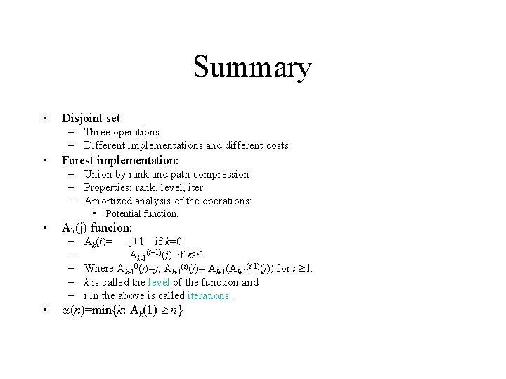
Summary • Disjoint set – Three operations – Different implementations and different costs • Forest implementation: – Union by rank and path compression – Properties: rank, level, iter. – Amortized analysis of the operations: • Potential function. • Ak(j) funcion: – – – • Ak(j)= j+1 if k=0 Ak-1(j+1)(j) if k 1 Where Ak-10(j)=j, Ak-1(i)(j)= Ak-1(i-1)(j)) for i 1. k is called the level of the function and i in the above is called iterations. (n)=min{k: Ak(1) n}

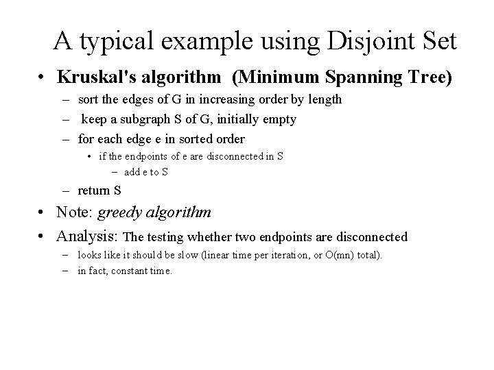
A typical example using Disjoint Set • Kruskal's algorithm (Minimum Spanning Tree) – sort the edges of G in increasing order by length – keep a subgraph S of G, initially empty – for each edge e in sorted order • if the endpoints of e are disconnected in S – add e to S – return S • Note: greedy algorithm • Analysis: The testing whether two endpoints are disconnected – looks like it should be slow (linear time per iteration, or O(mn) total). – in fact, constant time.