Lecture 19 Disjoint Sets CSE 373 Data Structures

Lecture 19: Disjoint Sets CSE 373: Data Structures and Algorithms CSE 373 2` SP – CHAMPION 1

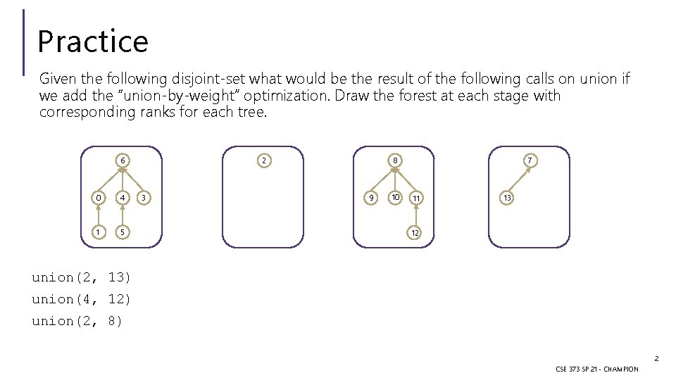
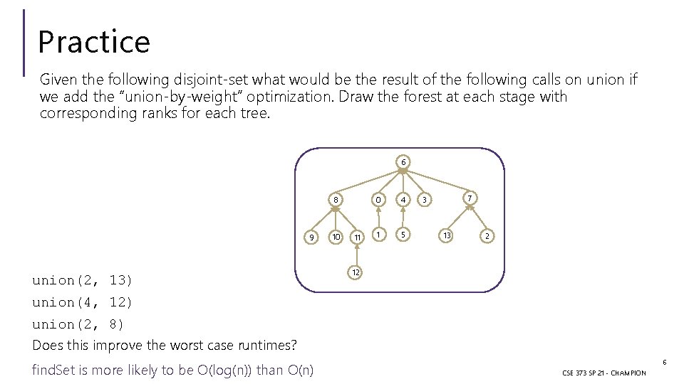
Practice Given the following disjoint-set what would be the result of the following calls on union if we add the “union-by-weight” optimization. Draw the forest at each stage with corresponding ranks for each tree. 6 0 4 1 5 2 3 8 9 10 7 11 13 12 union(2, 13) union(4, 12) union(2, 8) 2 CSE 373 SP 21 - CHAMPION

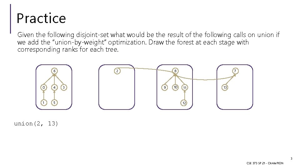
Practice Given the following disjoint-set what would be the result of the following calls on union if we add the “union-by-weight” optimization. Draw the forest at each stage with corresponding ranks for each tree. 6 0 4 1 5 2 3 8 9 10 7 11 13 12 union(2, 13) 3 CSE 373 SP 21 - CHAMPION

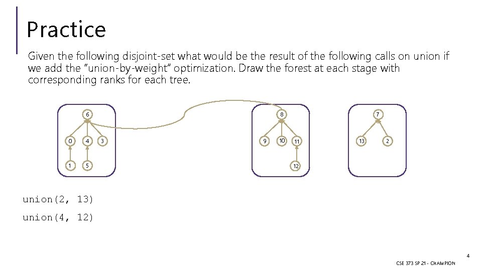
Practice Given the following disjoint-set what would be the result of the following calls on union if we add the “union-by-weight” optimization. Draw the forest at each stage with corresponding ranks for each tree. 6 0 4 1 5 8 3 9 10 7 11 13 2 12 union(2, 13) union(4, 12) 4 CSE 373 SP 21 - CHAMPION

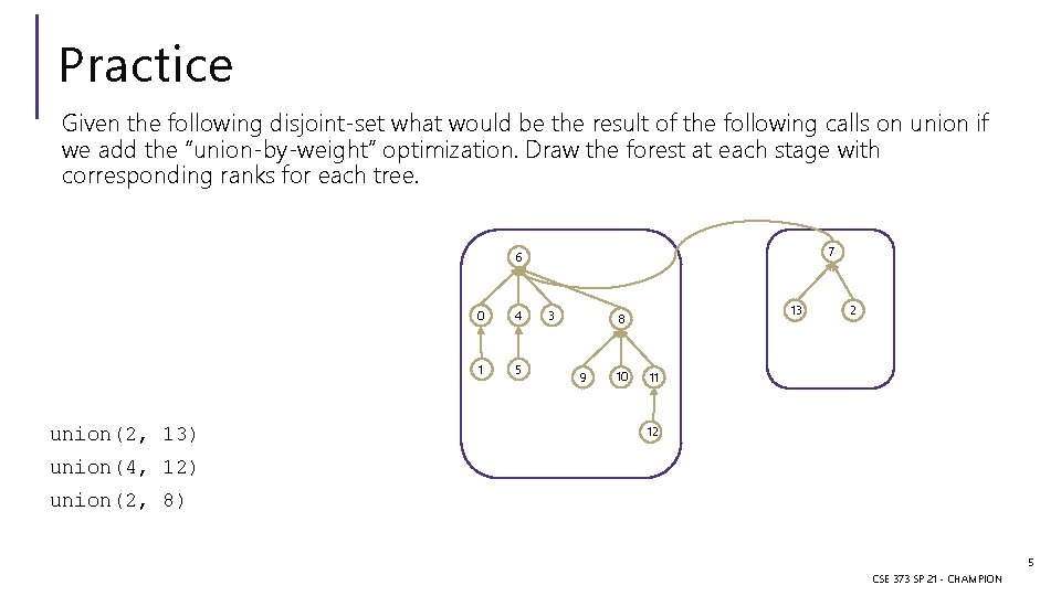
Practice Given the following disjoint-set what would be the result of the following calls on union if we add the “union-by-weight” optimization. Draw the forest at each stage with corresponding ranks for each tree. 7 6 union(2, 13) 0 4 1 5 3 13 8 9 10 2 11 12 union(4, 12) union(2, 8) 5 CSE 373 SP 21 - CHAMPION

Practice Given the following disjoint-set what would be the result of the following calls on union if we add the “union-by-weight” optimization. Draw the forest at each stage with corresponding ranks for each tree. 6 8 9 union(2, 13) 10 11 0 4 1 5 7 3 13 2 12 union(4, 12) union(2, 8) Does this improve the worst case runtimes? find. Set is more likely to be O(log(n)) than O(n) 6 CSE 373 SP 21 - CHAMPION

Midpoint survey Thank you all so much for filling out the lecture and section midpoint surveys! We appreciate the feedback and are working on incorporating it : )

Announcements P 3 due Today P 4 comes out today due in 3 weeks on Wednesday June 2 nd - last project! - ~2 weeks of work - extra credit spec quiz on gradescope! E 3 came out on Friday – due this Friday May 14 th - two more exercises coming Upcoming meme competition Reminders: - Tons of extra practice on section hand outs - section slides and videos are also available - always feel free to reach out to Tas

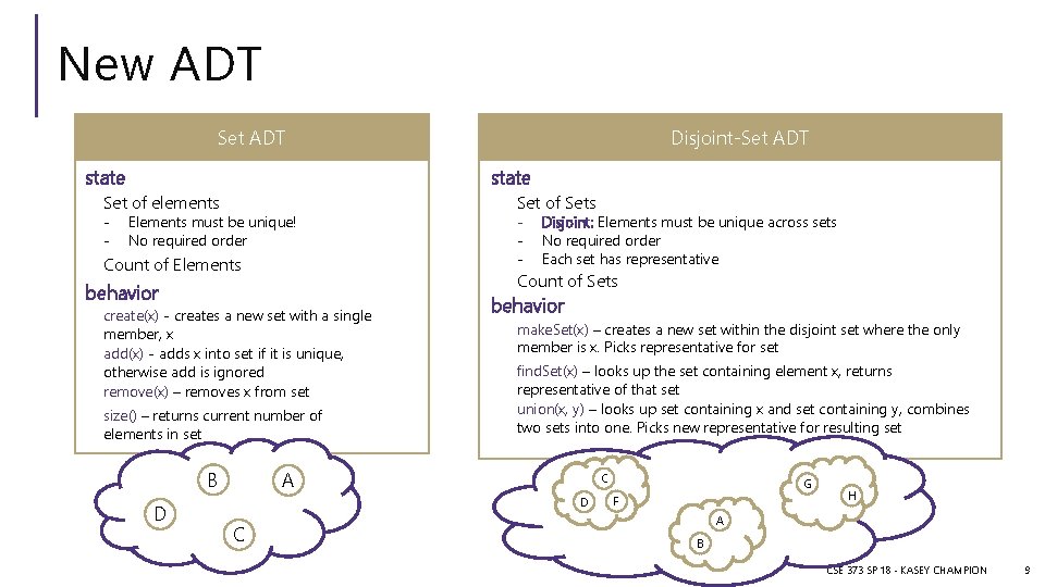
New ADT Set ADT state Set of elements - Disjoint-Set ADT Elements must be unique! No required order Count of Elements create(x) - creates a new set with a single member, x add(x) - adds x into set if it is unique, otherwise add is ignored remove(x) – removes x from set size() – returns current number of elements in set D - Disjoint: Elements must be unique across sets No required order Each set has representative Count of Sets behavior B Set of Sets behavior make. Set(x) – creates a new set within the disjoint set where the only member is x. Picks representative for set find. Set(x) – looks up the set containing element x, returns representative of that set union(x, y) – looks up set containing x and set containing y, combines two sets into one. Picks new representative for resulting set A C D C G F H A B CSE 373 SP 18 - KASEY CHAMPION 9

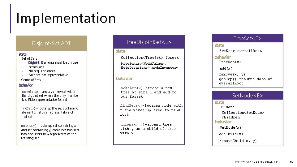
Implementation Tree. Disjoint. Set<E> Disjoint-Set ADT state Set of Sets Disjoint: Elements must be unique across sets No required order Each set has representative Count of Sets behavior make. Set(x) – creates a new set within the disjoint set where the only member is x. Picks representative for set find. Set(x) – looks up the set containing element x, returns representative of that set union(x, y) – looks up set containing x and set containing y, combines two sets into one. Picks new representative for resulting set state Collection<Tree. Set> forest Dictionary<Node. Values, Node. Locations> node. Inventory behavior Tree. Set<E> state Set. Node overall. Root behavior Tree. Set(x) add(x) remove(x, y) get. Rep()-returns data of overall. Root make. Set(x)-create a new tree of size 1 and add to our forest find. Set(x)-locates node with x and moves up tree to find root union(x, y)-append tree with y as a child of tree with x Set. Node<E> state E data Collection<Set. Node> children behavior Set. Node(x) add. Child(x) remove. Child(x, y) CSE 373 SP 18 - KASEY CHAMPION 10

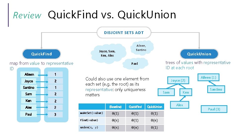
Review Quick. Find vs. Quick. Union DISJOINT SETS ADT Joyce, Sam, Ken, Alex Quick. Find map from value to representative ID Aileen 1 Joyce 2 Santino 1 Sam 2 Ken 2 Alex 2 Paul 3 Aileen, Santino Quick. Union trees of values with representative ID at each root Paul Could also use one element from each set (e. g. the root) as its representative: only uniqueness matters (Baseline) make. Set(value) find(value) union(x, y) Quick. Find Quick. Union Joyce (2) Sam Ken Alex Aileen (1) Santino Paul (3)

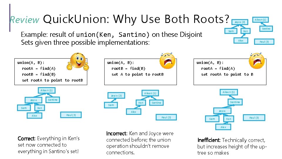
Quick. Union: Why Use Both Roots? Review union(A, B): root. A = find(A) root. B = find(B) set root. A to point to root. B union(A, B): root. B = find(B) set A to point to root. B Aileen (1) Santino Joyce Sam Alex Ken Sam Ken Paul (3) Alex Paul (3) union(A, B): root. A = find(A) set root. A to point to B Aileen (1) Joyce (2) Santino Ken Sam Example: result of union(Ken, Santino) on these Disjoint Sets given three possible implementations: Aileen (1) Joyce (2) Santino Joyce Alex Paul (3) Sam Ken Paul (3) Alex Correct: Everything in Ken’s set now connected to everything in Santino’s set! Incorrect: Ken and Joyce were connected before; the union operation shouldn’t remove connections. Inefficient: Technically correct, but increases height of the uptree so makes

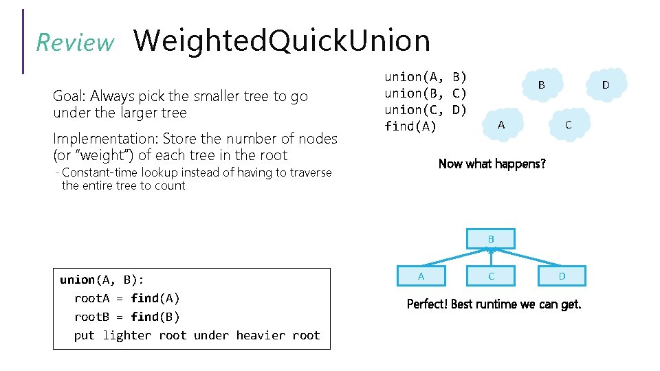
Review Weighted. Quick. Union Goal: Always pick the smaller tree to go under the larger tree Implementation: Store the number of nodes (or “weight”) of each tree in the root union(A, B) union(B, C) union(C, D) find(A) B A D C Now what happens? - Constant-time lookup instead of having to traverse the entire tree to count B union(A, B): root. A = find(A) root. B = find(B) put lighter root under heavier root A C D Perfect! Best runtime we can get.

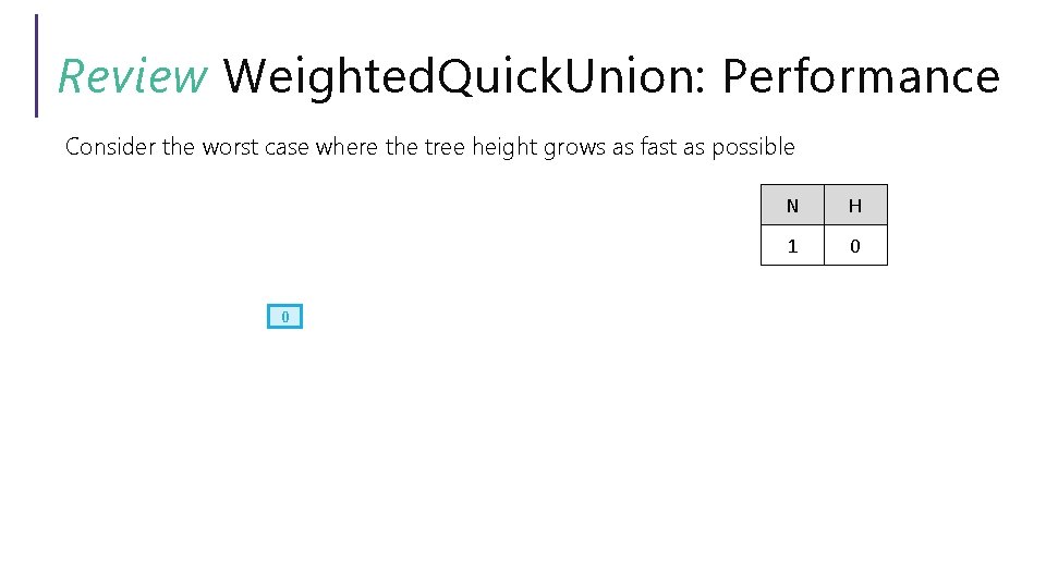
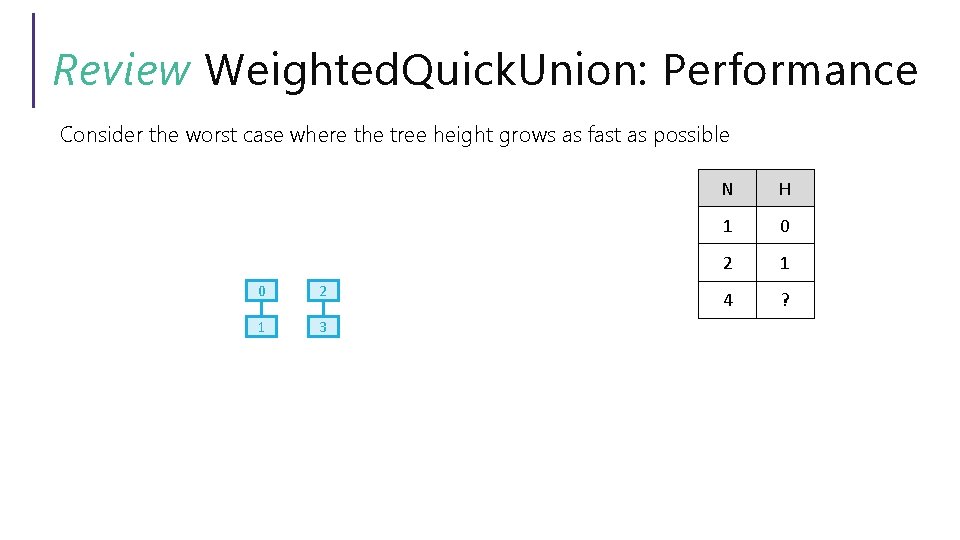
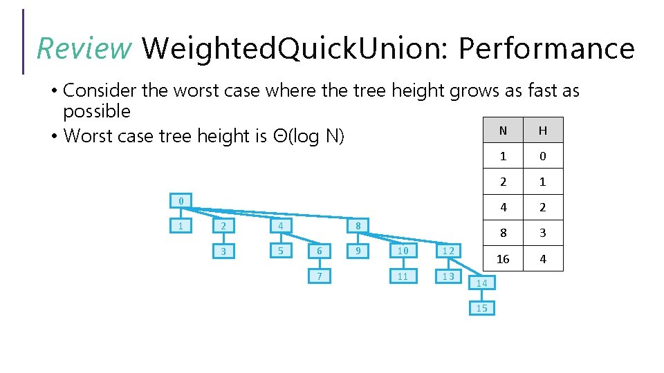
Review Weighted. Quick. Union: Performance Consider the worst case where the tree height grows as fast as possible 0 N H 1 0

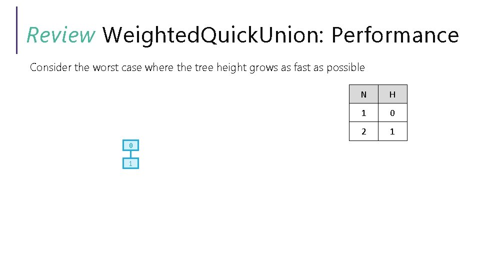
Review Weighted. Quick. Union: Performance Consider the worst case where the tree height grows as fast as possible 0 1 N H 1 0 2 1

Review Weighted. Quick. Union: Performance Consider the worst case where the tree height grows as fast as possible 0 2 1 3 N H 1 0 2 1 4 ?

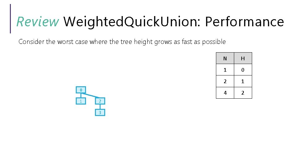
Review Weighted. Quick. Union: Performance Consider the worst case where the tree height grows as fast as possible 0 1 2 3 N H 1 0 2 1 4 2

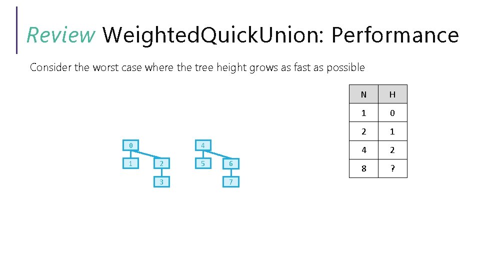
Review Weighted. Quick. Union: Performance Consider the worst case where the tree height grows as fast as possible 4 0 1 2 3 5 6 7 N H 1 0 2 1 4 2 8 ?

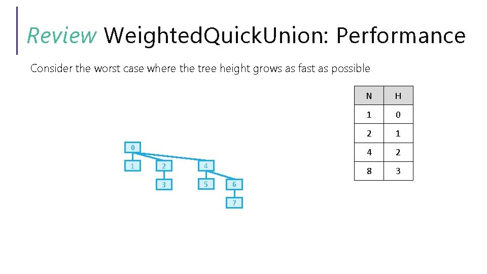
Review Weighted. Quick. Union: Performance Consider the worst case where the tree height grows as fast as possible 0 1 2 4 3 5 6 7 N H 1 0 2 1 4 2 8 3

Review Weighted. Quick. Union: Performance • Consider the worst case where the tree height grows as fast as possible N H • Worst case tree height is Θ(log N) 0 1 2 4 3 5 8 6 7 9 10 12 11 13 14 15 1 0 2 1 4 2 8 3 16 4

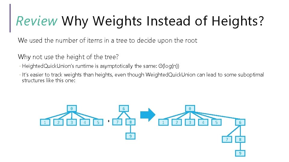
Review Why Weights Instead of Heights? We used the number of items in a tree to decide upon the root Why not use the height of the tree? - Heighted. Quick. Union’s runtime is asymptotically the same: Θ(log(n)) - It’s easier to track weights than heights, even though Weighted. Quick. Union can lead to some suboptimal structures like this one: 0 1 2 3 6 4 5 + 7 0 8 9 1 2 3 4 5 6 7 8 9

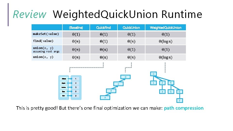
Review Weighted. Quick. Union Runtime (Baseline) Quick. Find Quick. Union Weighted. Quick. Union make. Set(value) find(value) union(x, y) assuming root args union(x, y) Aileen 1 Joyce 2 Santino 1 Sam 2 Ken 2 D C B A 0 1 2 4 3 5 6 7 This is pretty good! But there’s one final optimization we can make: path compression

Modifying Data Structures for Future Gains Thus far, the modifications we’ve studied are designed to preserve invariants - E. g. Performing rotations to preserve the AVL invariant - We rely on those invariants always being true so every call is fast Path compression is entirely different: we are modifying the tree structure to improve future performance - Not adhering to a specific invariant - The first call may be slow, but will optimize so future calls can be fast

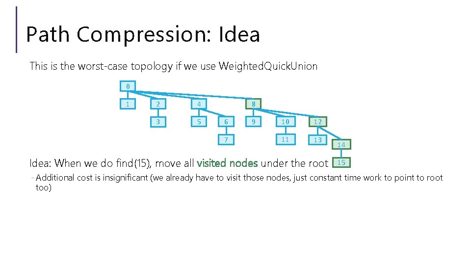
Path Compression: Idea This is the worst-case topology if we use Weighted. Quick. Union 0 1 2 4 3 5 8 6 7 9 10 12 11 13 Idea: When we do find(15), move all visited nodes under the root 14 15 - Additional cost is insignificant (we already have to visit those nodes, just constant time work to point to root too)

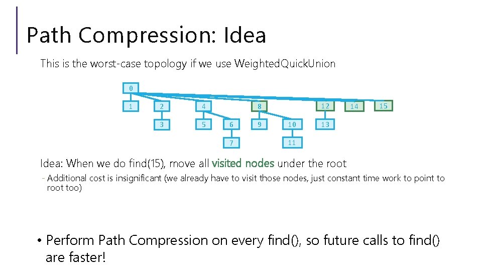
Path Compression: Idea This is the worst-case topology if we use Weighted. Quick. Union 0 1 2 4 3 5 12 8 6 7 9 10 14 15 13 11 Idea: When we do find(15), move all visited nodes under the root - Additional cost is insignificant (we already have to visit those nodes, just constant time work to point to root too) • Perform Path Compression on every find(), so future calls to find() are faster!

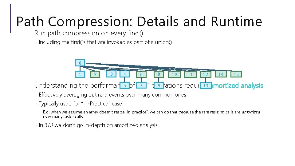
Path Compression: Details and Runtime Run path compression on every find()! - Including the find()s that are invoked as part of a union() 0 1 2 3 4 6 8 10 11 12 14 15 7 5 of M>1 9 13 amortized analysis Understanding the performance operations requires - Effectively averaging out rare events over many common ones - Typically used for “In-Practice” case - E. g. when we assume an array doesn’t resize “in practice”, we can do that because the rare resizing calls are amortized over many faster calls - In 373 we don’t go in-depth on amortized analysis

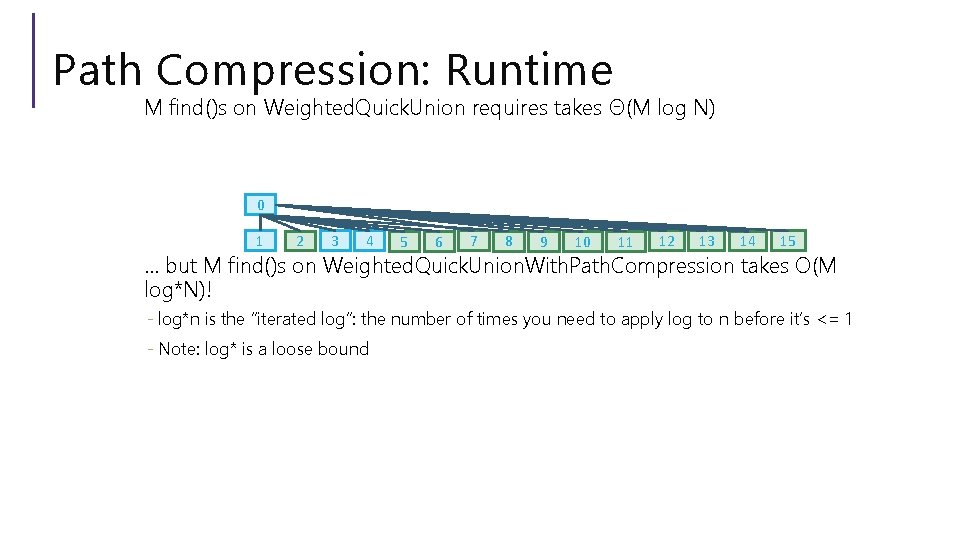
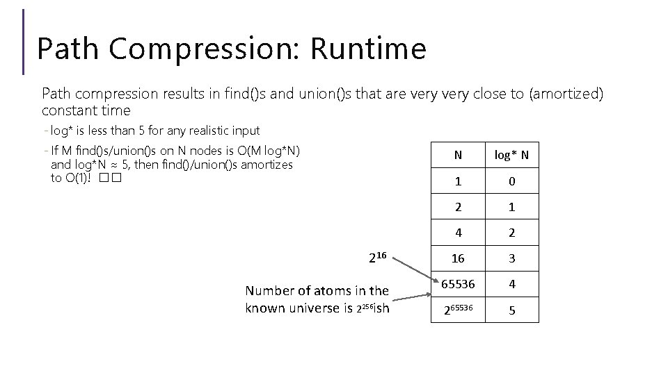
Path Compression: Runtime M find()s on Weighted. Quick. Union requires takes Θ(M log N) 0 1 2 3 4 5 6 7 8 9 10 11 12 13 14 15 … but M find()s on Weighted. Quick. Union. With. Path. Compression takes O(M log*N)! - log*n is the “iterated log”: the number of times you need to apply log to n before it’s <= 1 - Note: log* is a loose bound

Path Compression: Runtime Path compression results in find()s and union()s that are very close to (amortized) constant time - log* is less than 5 for any realistic input - If M find()s/union()s on N nodes is O(M log*N) and log*N ≈ 5, then find()/union()s amortizes to O(1)! �� 216 Number of atoms in the known universe is 2256 ish N log* N 1 0 2 1 4 2 16 3 65536 4 265536 5

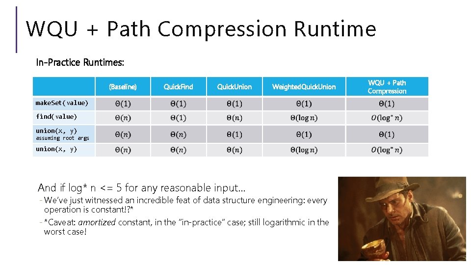
WQU + Path Compression Runtime In-Practice Runtimes: (Baseline) Quick. Find Quick. Union Weighted. Quick. Union make. Set(value) find(value) union(x, y) assuming root args union(x, y) And if log* n <= 5 for any reasonable input… - We’ve just witnessed an incredible feat of data structure engineering: every operation is constant!? * - *Caveat: amortized constant, in the “in-practice” case; still logarithmic in the worst case! WQU + Path Compression

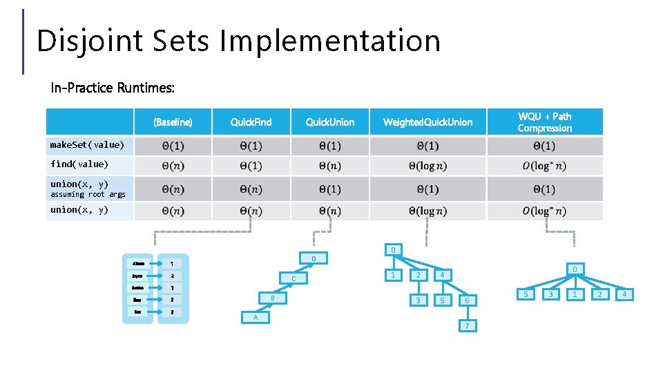
Disjoint Sets Implementation In-Practice Runtimes: (Baseline) Quick. Find Quick. Union Weighted. Quick. Union WQU + Path Compression make. Set(value) find(value) union(x, y) assuming root args union(x, y) Aileen 1 Joyce 2 Santino 1 Sam 2 Ken 2 D C B A 0 1 2 4 3 5 0 6 7 5 3 1 2 4

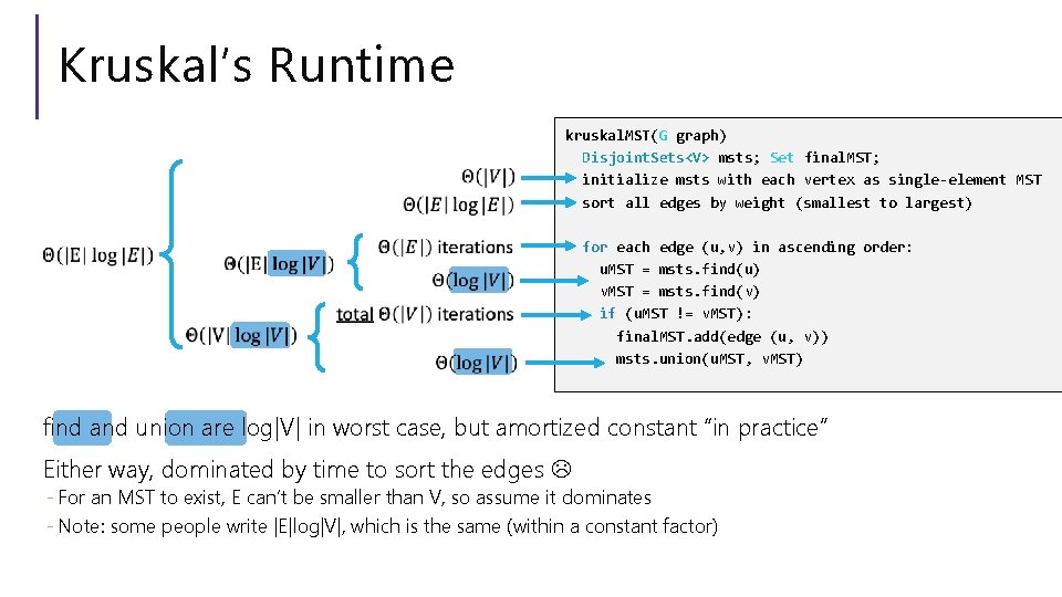
Kruskal’s Runtime kruskal. MST(G graph) Disjoint. Sets<V> msts; Set final. MST; initialize msts with each vertex as single-element MST sort all edges by weight (smallest to largest) for each edge (u, v) in ascending order: u. MST = msts. find(u) v. MST = msts. find(v) if (u. MST != v. MST): final. MST. add(edge (u, v)) msts. union(u. MST, v. MST) find and union are log|V| in worst case, but amortized constant “in practice” Either way, dominated by time to sort the edges - For an MST to exist, E can’t be smaller than V, so assume it dominates - Note: some people write |E|log|V|, which is the same (within a constant factor)

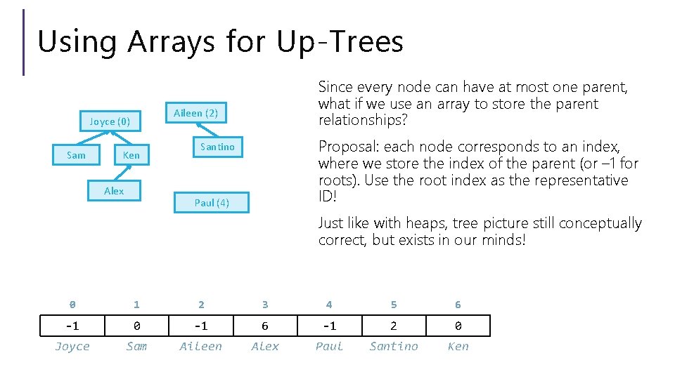
Using Arrays for Up-Trees Aileen (2) Joyce (0) Sam Since every node can have at most one parent, what if we use an array to store the parent relationships? Ken Alex Proposal: each node corresponds to an index, where we store the index of the parent (or – 1 for roots). Use the root index as the representative ID! Santino Paul (4) Just like with heaps, tree picture still conceptually correct, but exists in our minds! 0 1 2 3 4 5 6 -1 0 -1 6 -1 2 0 Joyce Sam Aileen Alex Paul Santino Ken

Using Arrays: Find find(A): index = jump to A node’s index 1 while array[index] > 0: 2 index = array[index] path compression 3 return index Initial jump to element still done with extra Map But traversing up the tree can be done purely within the array! • Can still do path compression by setting all indices along the way to the root index! Joyce (0) Alex Aileen Sam … Ken Sam 1 find(Alex) 1 2 3 -1 0 -1 6 0 Joyce Sam Aileen Alex 3 Santino = 0 Alex 0 Aileen (2) 4 5 6 -1 2 0 Paul Santino Ken 2 Paul (4)

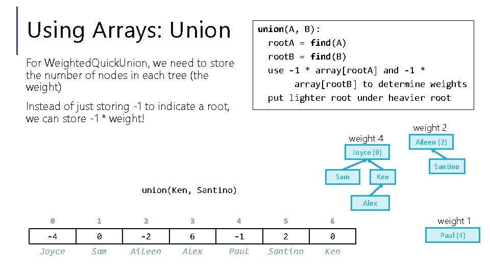
Using Arrays: Union union(A, B): root. A = find(A) root. B = find(B) use -1 * array[root. A] and -1 * array[root. B] to determine weights put lighter root under heavier root For Weighted. Quick. Union, we need to store the number of nodes in each tree (the weight) Instead of just storing -1 to indicate a root, we can store -1 * weight! weight 4 weight 2 Aileen (2) Joyce (0) Santino Sam Ken union(Ken, Santino) Alex 0 1 2 3 4 5 6 weight 1 -4 0 -2 6 -1 2 0 Paul (4) Joyce Sam Aileen Alex Paul Santino Ken

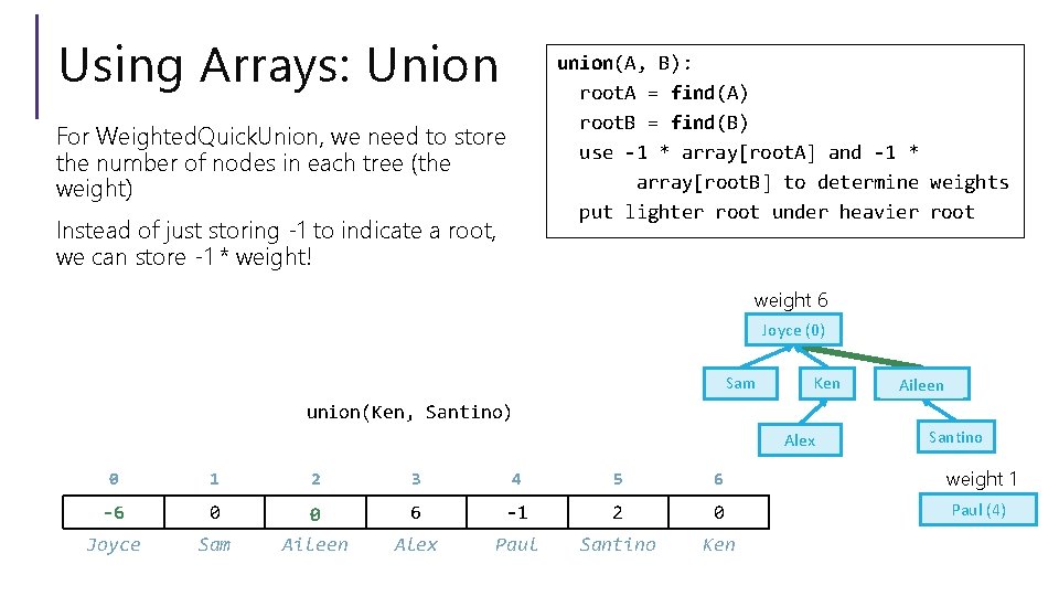
Using Arrays: Union union(A, B): root. A = find(A) root. B = find(B) use -1 * array[root. A] and -1 * array[root. B] to determine weights put lighter root under heavier root For Weighted. Quick. Union, we need to store the number of nodes in each tree (the weight) Instead of just storing -1 to indicate a root, we can store -1 * weight! weight 6 Joyce (0) Sam Ken Aileen(2) union(Ken, Santino) Alex Santino 0 1 2 3 4 5 6 weight 1 -4 -6 0 -2 0 6 -1 2 0 Paul (4) Joyce Sam Aileen Alex Paul Santino Ken

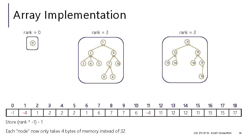
Array Implementation rank = 0 rank = 3 11 1 0 4 3 5 7 8 15 12 6 2 13 10 14 16 17 18 9 0 1 2 3 4 5 6 7 8 9 10 11 12 13 14 15 16 17 18 -1 -1 -4 1 2 2 2 1 6 7 7 6 -1 -4 11 12 12 11 15 15 17 Store (rank * -1) - 1 Each “node” now only takes 4 bytes of memory instead of 32 CSE 373 SP 18 - KASEY CHAMPION 36

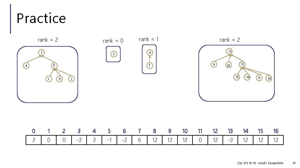
Practice rank = 2 rank = 0 3 rank = 1 0 1 13 6 5 4 rank = 2 9 7 11 12 10 15 2 14 8 16 0 1 2 3 4 5 6 7 8 9 10 11 12 13 14 15 16 3 0 0 -3 3 -1 -2 6 12 13 13 0 13 -3 12 12 12 CSE 373 SP 18 - KASEY CHAMPION 37

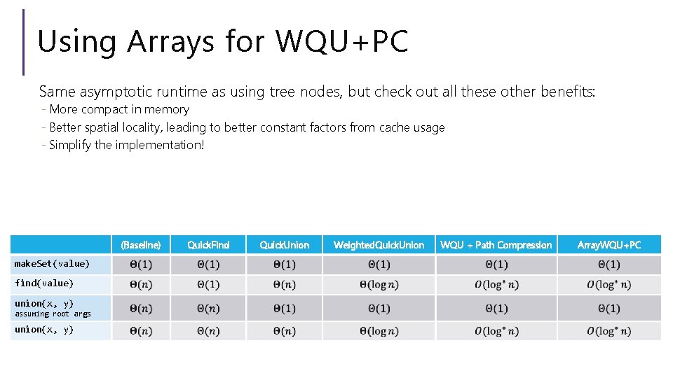
Using Arrays for WQU+PC Same asymptotic runtime as using tree nodes, but check out all these other benefits: - More compact in memory - Better spatial locality, leading to better constant factors from cache usage - Simplify the implementation! (Baseline) make. Set(value) find(value) union(x, y) assuming root args union(x, y) Quick. Find Quick. Union Weighted. Quick. Union WQU + Path Compression Array. WQU+PC

Appendix