Design and Analysis of Algorithms Khawaja Mohiuddin Assistant

Design and Analysis of Algorithms Khawaja Mohiuddin Assistant Professor, Department of Computer Sciences Bahria University, Karachi Campus, Contact: khawaja. mohiuddin@bimcs. edu. pk Lecture # 12 -13 – Greedy Method and Dynamic Programming CSC-305 Design and Analysis of Algorithms CSC-305 Design and Analysis of Algorithms BS(CS) -6 Fall-2014

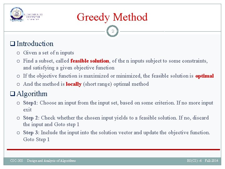
Greedy Method 2 q Introduction Given a set of n inputs Find a subset, called feasible solution, of the n inputs subject to some constraints, and satisfying a given objective function If the objective function is maximized or minimized, the feasible solution is optimal And the method is locally (short range) optimal method q Algorithm Step 1: Choose an input from the input set, based on some criterion. If no more input exit Step 2: Check whether the chosen input yields to a feasible solution. If no, discard the input and Goto step 1 Step 3: Include the input into the solution vector and update the objective function. Goto Step 1 CSC-305 Design and Analysis of Algorithms BS(CS) -6 Fall-2014

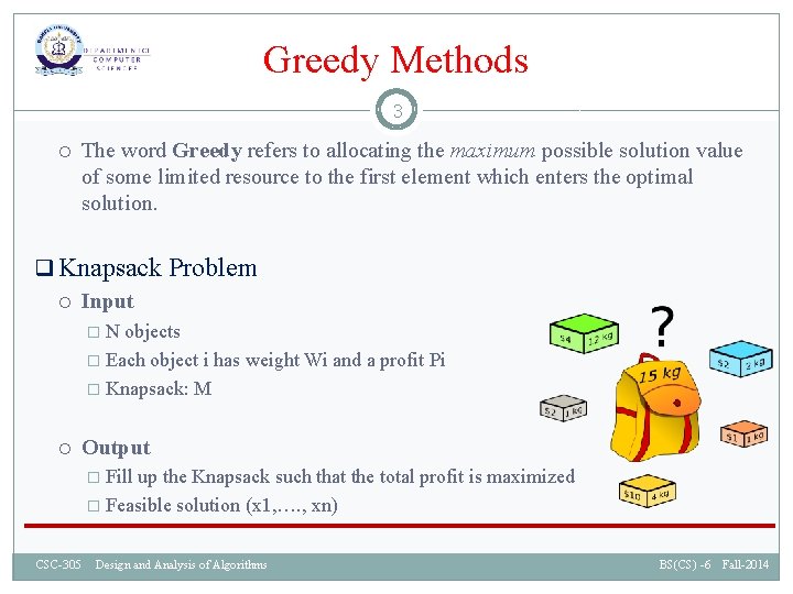
Greedy Methods 3 The word Greedy refers to allocating the maximum possible solution value of some limited resource to the first element which enters the optimal solution. q Knapsack Problem Input � N objects � Each object i has weight Wi and a profit Pi � Knapsack: M Output � Fill up the Knapsack such that the total profit is maximized � Feasible solution (x 1, …. , xn) CSC-305 Design and Analysis of Algorithms BS(CS) -6 Fall-2014

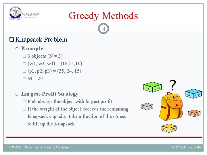
Greedy Methods 4 q Knapsack Problem Example � 3 objects (N = 3) � (w 1, w 2, w 3) = (18, 15, 10) � (p 1, p 2, p 3) = (25, 24, 15) � M = 20 Largest-Profit Strategy � Pick always the object with largest profit � If the weight of the object exceeds the remaining Knapsack capacity, take a fraction of the object to fill up the Knapsack CSC-305 Design and Analysis of Algorithms BS(CS) -6 Fall-2014

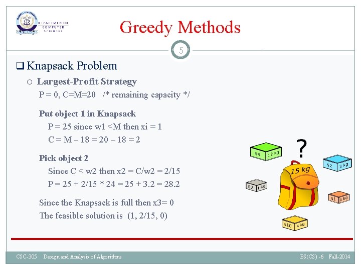
Greedy Methods 5 q Knapsack Problem Largest-Profit Strategy P = 0, C=M=20 /* remaining capacity */ Put object 1 in Knapsack P = 25 since w 1 <M then xi = 1 C = M – 18 = 20 – 18 = 2 Pick object 2 Since C < w 2 then x 2 = C/w 2 = 2/15 P = 25 + 2/15 * 24 = 25 + 3. 2 = 28. 2 Since the Knapsack is full then x 3= 0 The feasible solution is (1, 2/15, 0) CSC-305 Design and Analysis of Algorithms BS(CS) -6 Fall-2014

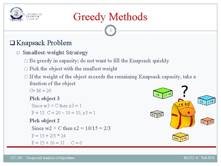
Greedy Methods 6 q Knapsack Problem Smallest-weight Strategy � Be greedy in capacity; do not want to fill the Knapsack quickly � Pick the object with the smallest weight � If the weight of the object exceeds the remaining Knapsack capacity, take a fraction of the object C= M = 20 Pick object 3 Since w 3 < C then x 3 = 1 P = 15 C = 20 – 10 = 10, x 3 = 1 Pick object 2 Since w 2 > C then x 2 = 10/15 = 2/3 P = 15 + 2/3 * 24 P = 15 + 16 = 31 C = 0 CSC-305 Design and Analysis of Algorithms BS(CS) -6 Fall-2014

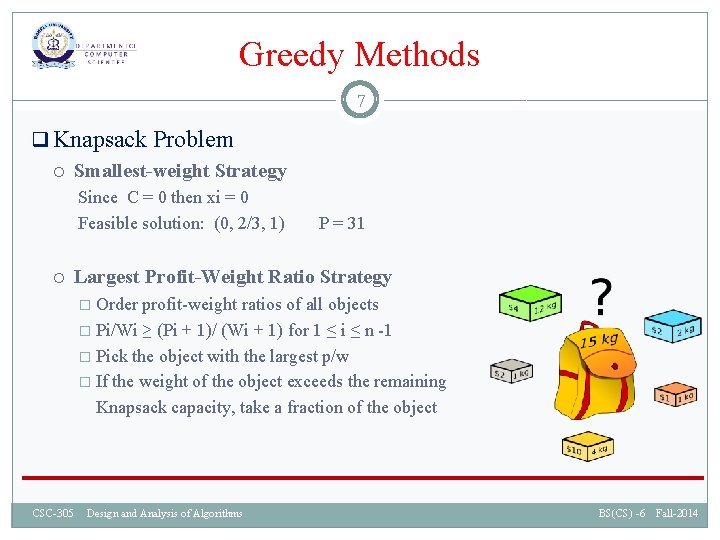
Greedy Methods 7 q Knapsack Problem Smallest-weight Strategy Since C = 0 then xi = 0 Feasible solution: (0, 2/3, 1) P = 31 Largest Profit-Weight Ratio Strategy � Order profit-weight ratios of all objects � Pi/Wi ≥ (Pi + 1)/ (Wi + 1) for 1 ≤ i ≤ n -1 � Pick the object with the largest p/w � If the weight of the object exceeds the remaining Knapsack capacity, take a fraction of the object CSC-305 Design and Analysis of Algorithms BS(CS) -6 Fall-2014

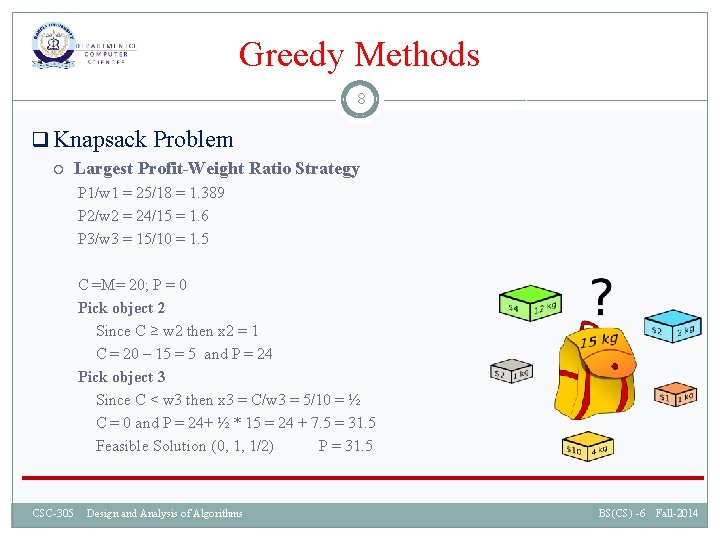
Greedy Methods 8 q Knapsack Problem Largest Profit-Weight Ratio Strategy P 1/w 1 = 25/18 = 1. 389 P 2/w 2 = 24/15 = 1. 6 P 3/w 3 = 15/10 = 1. 5 C =M= 20; P = 0 Pick object 2 Since C ≥ w 2 then x 2 = 1 C = 20 – 15 = 5 and P = 24 Pick object 3 Since C < w 3 then x 3 = C/w 3 = 5/10 = ½ C = 0 and P = 24+ ½ * 15 = 24 + 7. 5 = 31. 5 Feasible Solution (0, 1, 1/2) P = 31. 5 CSC-305 Design and Analysis of Algorithms BS(CS) -6 Fall-2014

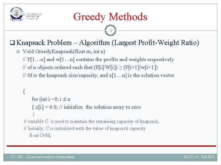
Greedy Methods 9 q Knapsack Problem – Algorithm (Largest Profit-Weight Ratio) Void Greedy. Knapsack(float m, int n) // P[1…n] and w[1…n] contains the profits and weights respectively // of n objects ordered such that (P[i]/W[i]) ≥ (P[i+1]/w[i+1]) // M is the knapsack size/capacity, and x[1…n] is the solution vector { for (int i =0; i ≤ n { x[i] = 0. 0; // initialize the solution array to zero } // variable C is used to maintain the remaining capacity of knapsack; // Initially, C is initialized with the value of knapsack capacity float C=M; CSC-305 Design and Analysis of Algorithms BS(CS) -6 Fall-2014

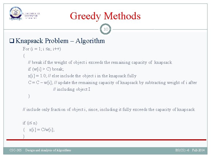
Greedy Methods 10 q Knapsack Problem – Algorithm For (i = 1; i ≤n; i++) { // break if the weight of object i exceeds the remaining capacity of knapsack if (w[i] > C) break; x[i] = 1. 0; // else include the object i in the knapsack fully C = C – w[i]; // update the remaining capacity of knapsack by subtracting weight of i after // including object I } // include only fraction of object i, since, including it fully exceeds the capacity of knapsack if (i≤ n) { x[i] = C/w[i]; } CSC-305 Design and Analysis of Algorithms BS(CS) -6 Fall-2014

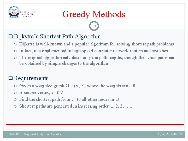
Greedy Methods 11 q Dijkstra’s Shortest Path Algorithm Dijkstra is well-known and a popular algorithm for solving shortest path problems In fact, it is implemented in high-speed computer network routers and switches The original algorithm calculates only the path lengths, though the actual paths can be obtained by simple changes to the algorithm q Requirements Given a weighted graph G = (V, E) where the weights are > 0 A source vertex, v 0 ϵ V Find the shortest path from v 0 to all other nodes in G Shortest paths are generated in increasing order: 1, 2, 3, …. . CSC-305 Design and Analysis of Algorithms BS(CS) -6 Fall-2014

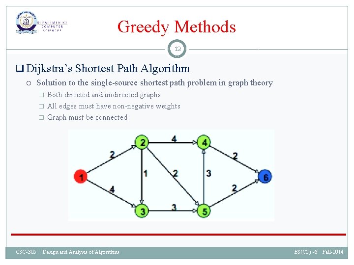
Greedy Methods 12 q Dijkstra’s Shortest Path Algorithm Solution to the single-source shortest path problem in graph theory � � � Both directed and undirected graphs All edges must have non-negative weights Graph must be connected CSC-305 Design and Analysis of Algorithms BS(CS) -6 Fall-2014

Greedy Methods 13 q Dijkstra’s Shortest Path Algorithm function Dijkstra(Graph, source): dist[source] : = 0 // Distance from source to source for each vertex v in Graph: // Initializations if v != source dist[v] : = infinity // Unknown distance function from source to v previous[v] : = undefined // Previous node in optimal path from source end if add v to Q // All nodes initially in Q (unvisited nodes) end for (continued on next slide) CSC-305 Design and Analysis of Algorithms BS(CS) -6 Fall-2014

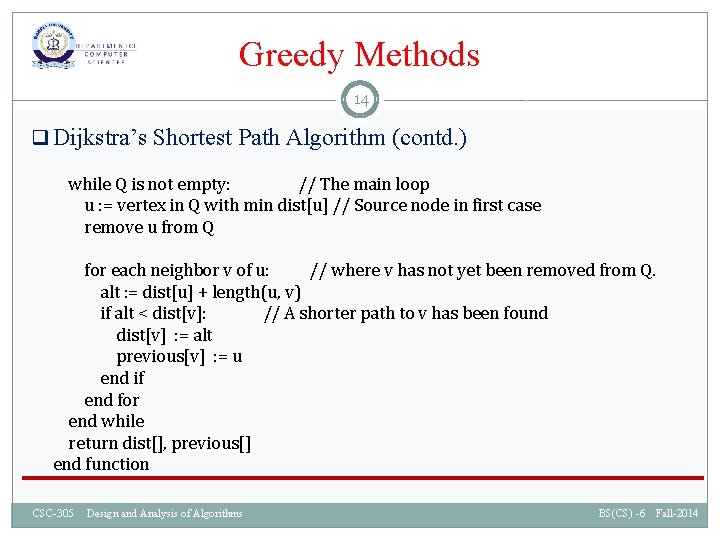
Greedy Methods 14 q Dijkstra’s Shortest Path Algorithm (contd. ) while Q is not empty: // The main loop u : = vertex in Q with min dist[u] // Source node in first case remove u from Q for each neighbor v of u: // where v has not yet been removed from Q. alt : = dist[u] + length(u, v) if alt < dist[v]: // A shorter path to v has been found dist[v] : = alt previous[v] : = u end if end for end while return dist[], previous[] end function CSC-305 Design and Analysis of Algorithms BS(CS) -6 Fall-2014

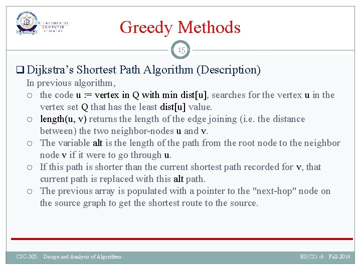
Greedy Methods 15 q Dijkstra’s Shortest Path Algorithm (Description) In previous algorithm, the code u : = vertex in Q with min dist[u], searches for the vertex u in the vertex set Q that has the least dist[u] value. length(u, v) returns the length of the edge joining (i. e. the distance between) the two neighbor-nodes u and v. The variable alt is the length of the path from the root node to the neighbor node v if it were to go through u. If this path is shorter than the current shortest path recorded for v, that current path is replaced with this alt path. The previous array is populated with a pointer to the "next-hop" node on the source graph to get the shortest route to the source. CSC-305 Design and Analysis of Algorithms BS(CS) -6 Fall-2014

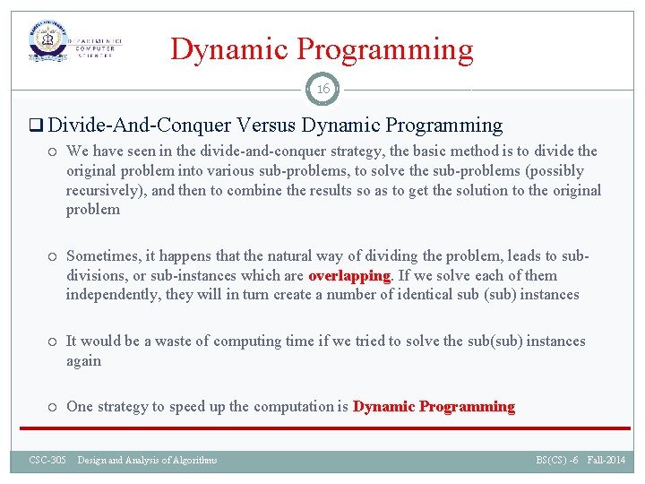
Dynamic Programming 16 q Divide-And-Conquer Versus Dynamic Programming We have seen in the divide-and-conquer strategy, the basic method is to divide the original problem into various sub-problems, to solve the sub-problems (possibly recursively), and then to combine the results so as to get the solution to the original problem Sometimes, it happens that the natural way of dividing the problem, leads to subdivisions, or sub-instances which are overlapping. If we solve each of them independently, they will in turn create a number of identical sub (sub) instances It would be a waste of computing time if we tried to solve the sub(sub) instances again One strategy to speed up the computation is Dynamic Programming CSC-305 Design and Analysis of Algorithms BS(CS) -6 Fall-2014

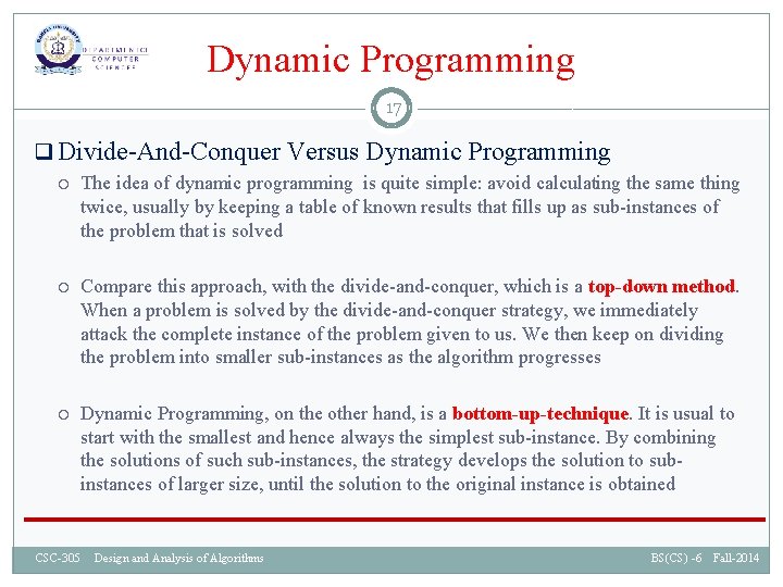
Dynamic Programming 17 q Divide-And-Conquer Versus Dynamic Programming The idea of dynamic programming is quite simple: avoid calculating the same thing twice, usually by keeping a table of known results that fills up as sub-instances of the problem that is solved Compare this approach, with the divide-and-conquer, which is a top-down method. When a problem is solved by the divide-and-conquer strategy, we immediately attack the complete instance of the problem given to us. We then keep on dividing the problem into smaller sub-instances as the algorithm progresses Dynamic Programming, on the other hand, is a bottom-up-technique. It is usual to start with the smallest and hence always the simplest sub-instance. By combining the solutions of such sub-instances, the strategy develops the solution to subinstances of larger size, until the solution to the original instance is obtained CSC-305 Design and Analysis of Algorithms BS(CS) -6 Fall-2014

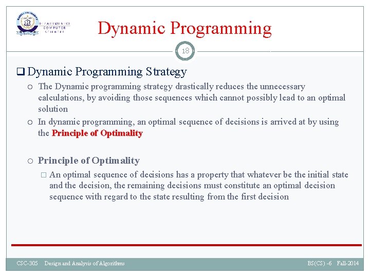
Dynamic Programming 18 q Dynamic Programming Strategy The Dynamic programming strategy drastically reduces the unnecessary calculations, by avoiding those sequences which cannot possibly lead to an optimal solution In dynamic programming, an optimal sequence of decisions is arrived at by using the Principle of Optimality � An optimal sequence of decisions has a property that whatever be the initial state and the decision, the remaining decisions must constitute an optimal decision sequence with regard to the state resulting from the first decision CSC-305 Design and Analysis of Algorithms BS(CS) -6 Fall-2014

Dynamic Programming 19 q Dynamic Programming Strategy There are four steps in a dynamic programming solution: 1. Characterise the structure of an optimal solution 2. Define recursively the value of an optimal solution 3. Compute the value of an optimal solution in a bottom-up fashion 4. Construct an optimal solution from the computed information CSC-305 Design and Analysis of Algorithms BS(CS) -6 Fall-2014

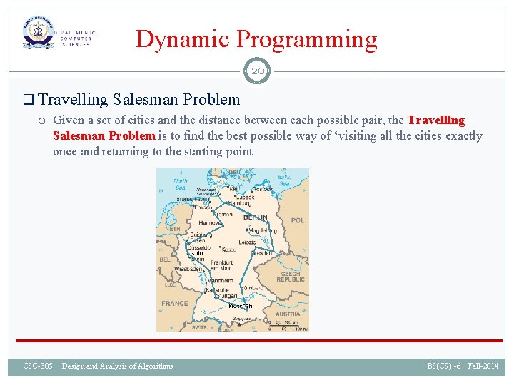
Dynamic Programming 20 q Travelling Salesman Problem Given a set of cities and the distance between each possible pair, the Travelling Salesman Problem is to find the best possible way of ‘visiting all the cities exactly once and returning to the starting point CSC-305 Design and Analysis of Algorithms BS(CS) -6 Fall-2014

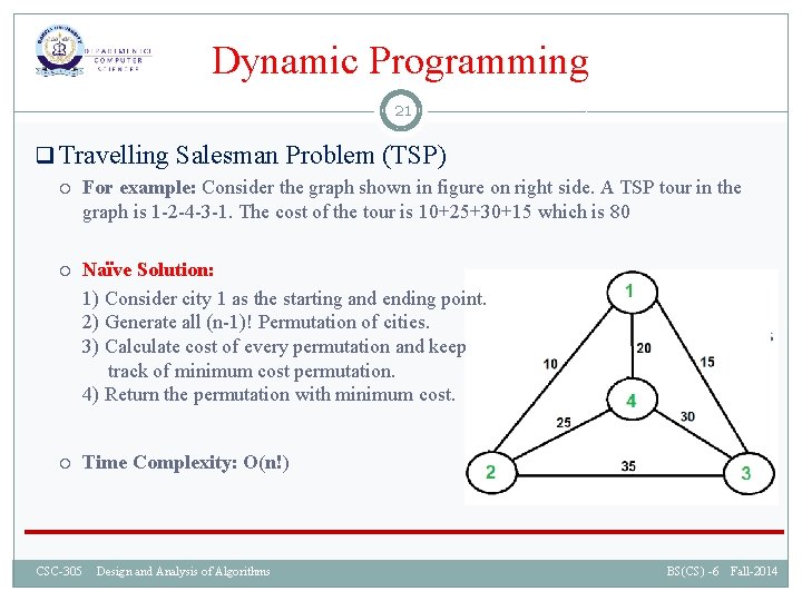
Dynamic Programming 21 q Travelling Salesman Problem (TSP) For example: Consider the graph shown in figure on right side. A TSP tour in the graph is 1 -2 -4 -3 -1. The cost of the tour is 10+25+30+15 which is 80 Naïve Solution: 1) Consider city 1 as the starting and ending point. 2) Generate all (n-1)! Permutation of cities. 3) Calculate cost of every permutation and keep track of minimum cost permutation. 4) Return the permutation with minimum cost. Time Complexity: O(n!) CSC-305 Design and Analysis of Algorithms BS(CS) -6 Fall-2014

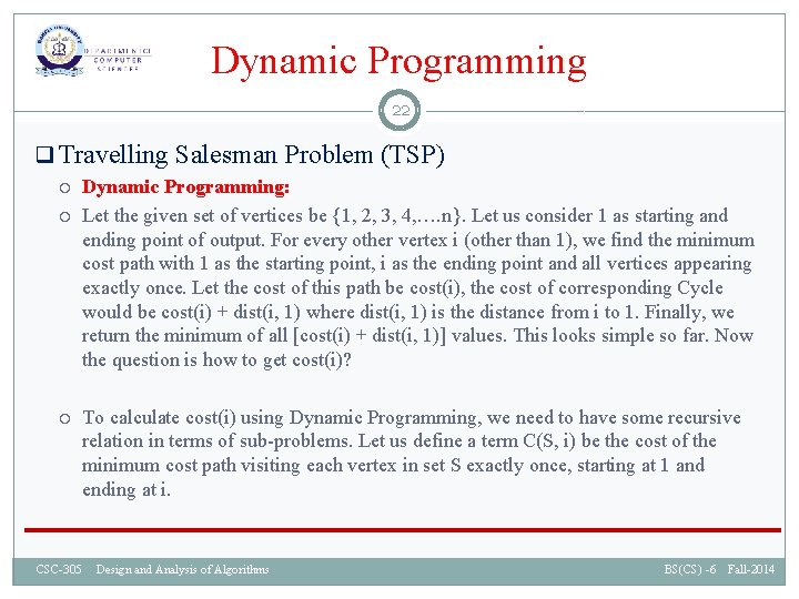
Dynamic Programming 22 q Travelling Salesman Problem (TSP) Dynamic Programming: Let the given set of vertices be {1, 2, 3, 4, …. n}. Let us consider 1 as starting and ending point of output. For every other vertex i (other than 1), we find the minimum cost path with 1 as the starting point, i as the ending point and all vertices appearing exactly once. Let the cost of this path be cost(i), the cost of corresponding Cycle would be cost(i) + dist(i, 1) where dist(i, 1) is the distance from i to 1. Finally, we return the minimum of all [cost(i) + dist(i, 1)] values. This looks simple so far. Now the question is how to get cost(i)? To calculate cost(i) using Dynamic Programming, we need to have some recursive relation in terms of sub-problems. Let us define a term C(S, i) be the cost of the minimum cost path visiting each vertex in set S exactly once, starting at 1 and ending at i. CSC-305 Design and Analysis of Algorithms BS(CS) -6 Fall-2014

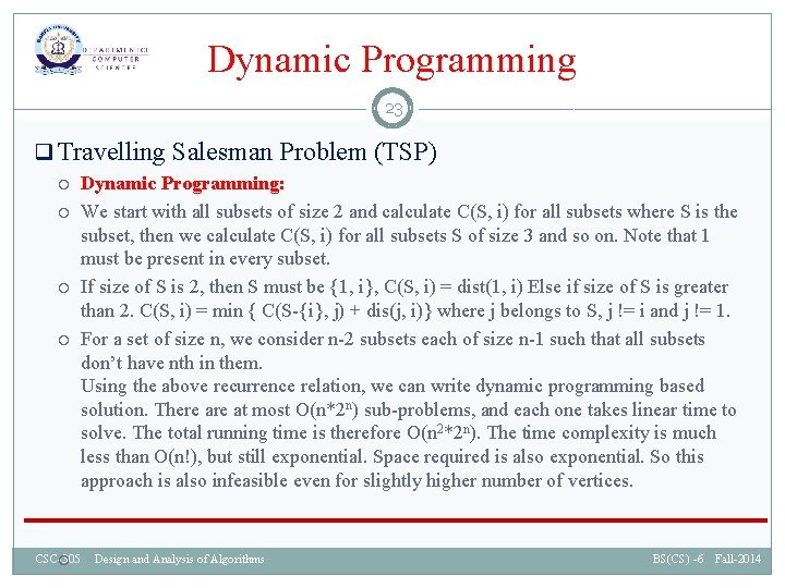
Dynamic Programming 23 q Travelling Salesman Problem (TSP) Dynamic Programming: We start with all subsets of size 2 and calculate C(S, i) for all subsets where S is the subset, then we calculate C(S, i) for all subsets S of size 3 and so on. Note that 1 must be present in every subset. If size of S is 2, then S must be {1, i}, C(S, i) = dist(1, i) Else if size of S is greater than 2. C(S, i) = min { C(S-{i}, j) + dis(j, i)} where j belongs to S, j != i and j != 1. For a set of size n, we consider n-2 subsets each of size n-1 such that all subsets don’t have nth in them. Using the above recurrence relation, we can write dynamic programming based solution. There at most O(n*2 n) sub-problems, and each one takes linear time to solve. The total running time is therefore O(n 2*2 n). The time complexity is much less than O(n!), but still exponential. Space required is also exponential. So this approach is also infeasible even for slightly higher number of vertices. CSC-305 Design and Analysis of Algorithms BS(CS) -6 Fall-2014

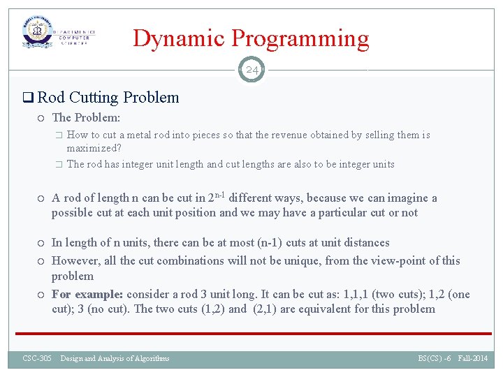
Dynamic Programming 24 q Rod Cutting Problem The Problem: � � How to cut a metal rod into pieces so that the revenue obtained by selling them is maximized? The rod has integer unit length and cut lengths are also to be integer units A rod of length n can be cut in 2 n-1 different ways, because we can imagine a possible cut at each unit position and we may have a particular cut or not In length of n units, there can be at most (n-1) cuts at unit distances However, all the cut combinations will not be unique, from the view-point of this problem For example: consider a rod 3 unit long. It can be cut as: 1, 1, 1 (two cuts); 1, 2 (one cut); 3 (no cut). The two cuts (1, 2) and (2, 1) are equivalent for this problem CSC-305 Design and Analysis of Algorithms BS(CS) -6 Fall-2014

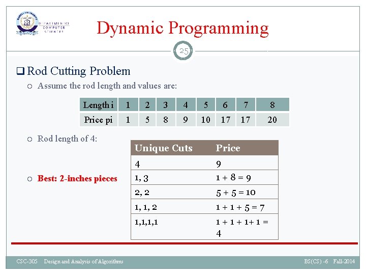
Dynamic Programming 25 q Rod Cutting Problem Assume the rod length and values are: Length i 1 2 3 4 5 6 7 8 Price pi 1 5 8 9 10 17 17 20 Rod length of 4: Best: 2 -inches pieces CSC-305 Design and Analysis of Algorithms Unique Cuts Price 4 9 1, 3 1+8=9 2, 2 5 + 5 = 10 1, 1, 2 1+1+5=7 1, 1, 1, 1 1 + 1+ 1 = 4 BS(CS) -6 Fall-2014

Dynamic Programming 26 q Rod Cutting Problem DP-CUT-ROD(p, n) let r[0. . n], s[0. . n] be new arrays r[0]=0 for j=1 to n q=-∞ for i=1 to j if q < p[i]+r[j-i] s[j]=i; q= p[i]+r[j-i] r[j]=q return r and s CSC-305 Design and Analysis of Algorithms BS(CS) -6 Fall-2014

Summary 27 q Greedy Methods Knapsack Problem Djikstra’s Shortest Path Algorithm q Dynamic Programming Travelling Salesman Problem Rod Cutting Problem CSC-305 Design and Analysis of Algorithms BS(CS) -6 Fall-2014