Data Warehousing and OLAP CENG 514 01 January

Data Warehousing and OLAP CENG 514 01 January 2022 1

Data Analysis Needs • Operational databases served as the source of information to facilitate the decision making process – Decision support systems (DSS) were developed around this data • Information requirements have grown quite complex over time and it is difficult to extract all the needed information from a database 01 January 2022 2

Decision Support Systems • Methodology (or series of methodologies) designed to extract information from data and to use such information as a basis for decision making • Decision support system (DSS): – Arrangement of computerized tools used to assist managerial decision making within a business – Used at all levels within an organization – Often tailored to focus on specific business areas – Provides ad hoc query tools to retrieve data and to display data in different formats 01 January 2022 3

Decision Support Systems • Combines historical operational data with business models that reflect the business activities – Compare the relative rates of productivity growth by company division over some specified period of time – Define the relationship between advertising types and sales levels – Define relative market shares by selected product lines 01 January 2022 4

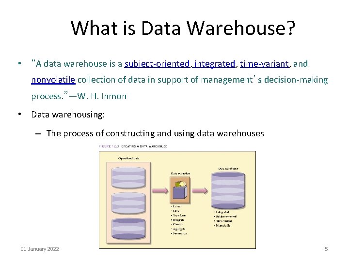
What is Data Warehouse? • “A data warehouse is a subject-oriented, integrated, time-variant, and nonvolatile collection of data in support of management’s decision-making process. ”—W. H. Inmon • Data warehousing: – The process of constructing and using data warehouses 01 January 2022 5

Data Warehouse—Subject-Oriented • Organized around major subjects, such as customer, product, sales. • Focusing on the modeling and analysis of data for decision makers, not on daily operations or transaction processing. • Provide a simple and concise view around particular subject issues by excluding data that are not useful in the decision support process. 01 January 2022 6

Data Warehouse—Integrated • Constructed by integrating multiple, heterogeneous data sources – relational databases, flat files, on-line transaction records • Data cleaning and data integration techniques are applied. – Ensure consistency in naming conventions, encoding structures, attribute measures, etc. among different data sources • E. g. , Hotel price: currency, tax, breakfast covered, etc. – When data is moved to the warehouse, it is converted. 01 January 2022 7

Data Warehouse—Time Variant • The time horizon for the data warehouse is significantly longer than that of operational systems. – Operational database: current value data. – Data warehouse data: provide information from a historical perspective (e. g. , past 5 -10 years) • Every key structure in the data warehouse – Contains an element of time, explicitly or implicitly – But the key of operational data may or may not contain “time element”. 01 January 2022 8

Data Warehouse—Non-Volatile • A physically separate store of data transformed from the operational environment. • Operational update of data does not occur in the data warehouse environment. – Does not require transaction processing, recovery, and concurrency control mechanisms – Requires only two operations in data accessing: • initial loading of data and access of data. 01 January 2022 9

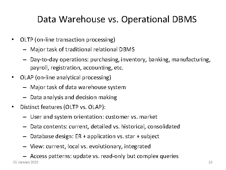
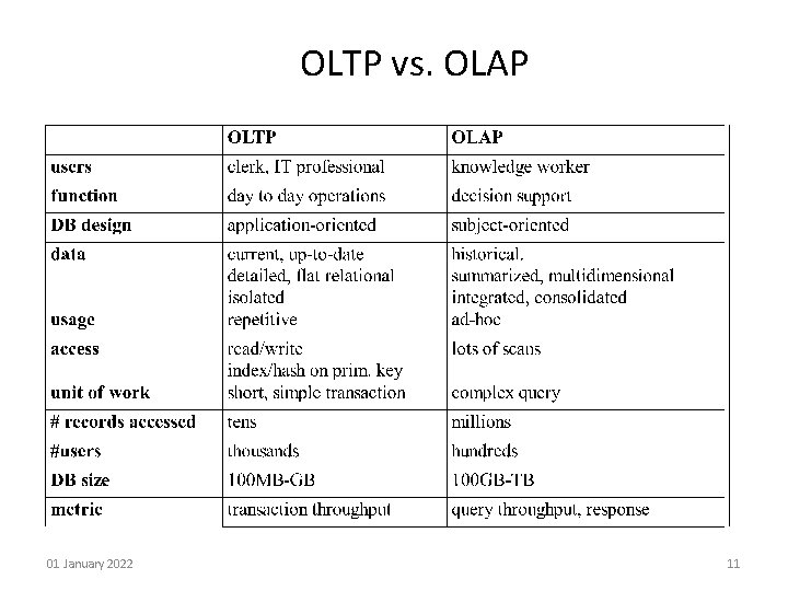
Data Warehouse vs. Operational DBMS • OLTP (on-line transaction processing) – Major task of traditional relational DBMS – Day-to-day operations: purchasing, inventory, banking, manufacturing, payroll, registration, accounting, etc. • OLAP (on-line analytical processing) – Major task of data warehouse system – Data analysis and decision making • Distinct features (OLTP vs. OLAP): – User and system orientation: customer vs. market – Data contents: current, detailed vs. historical, consolidated – Database design: ER + application vs. star + subject – View: current, local vs. evolutionary, integrated – Access patterns: update vs. read-only but complex queries 01 January 2022 10

OLTP vs. OLAP 01 January 2022 11

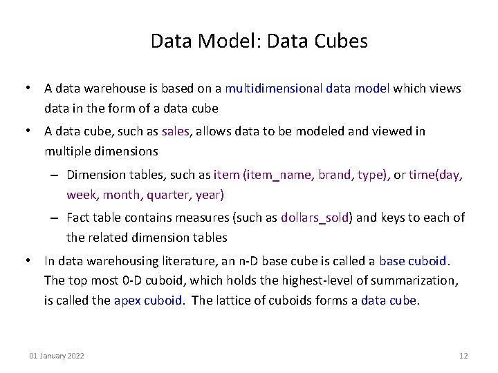
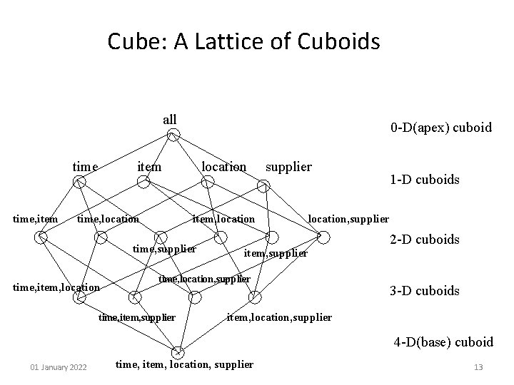
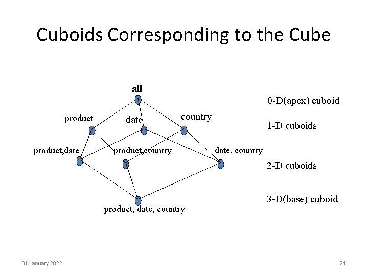
Data Model: Data Cubes • A data warehouse is based on a multidimensional data model which views data in the form of a data cube • A data cube, such as sales, allows data to be modeled and viewed in multiple dimensions – Dimension tables, such as item (item_name, brand, type), or time(day, week, month, quarter, year) – Fact table contains measures (such as dollars_sold) and keys to each of the related dimension tables • In data warehousing literature, an n-D base cube is called a base cuboid. The top most 0 -D cuboid, which holds the highest-level of summarization, is called the apex cuboid. The lattice of cuboids forms a data cube. 01 January 2022 12

Cube: A Lattice of Cuboids all time, item 0 -D(apex) cuboid item time, location item, location time, supplier time, item, location supplier location, supplier item, supplier time, location, supplier time, item, supplier 1 -D cuboids 2 -D cuboids 3 -D cuboids item, location, supplier 4 -D(base) cuboid 01 January 2022 time, item, location, supplier 13

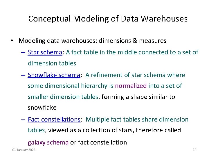
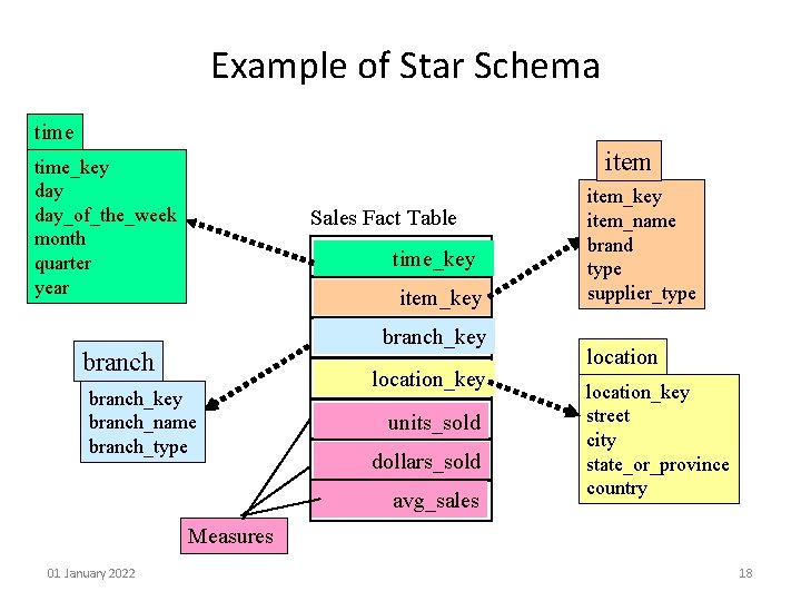
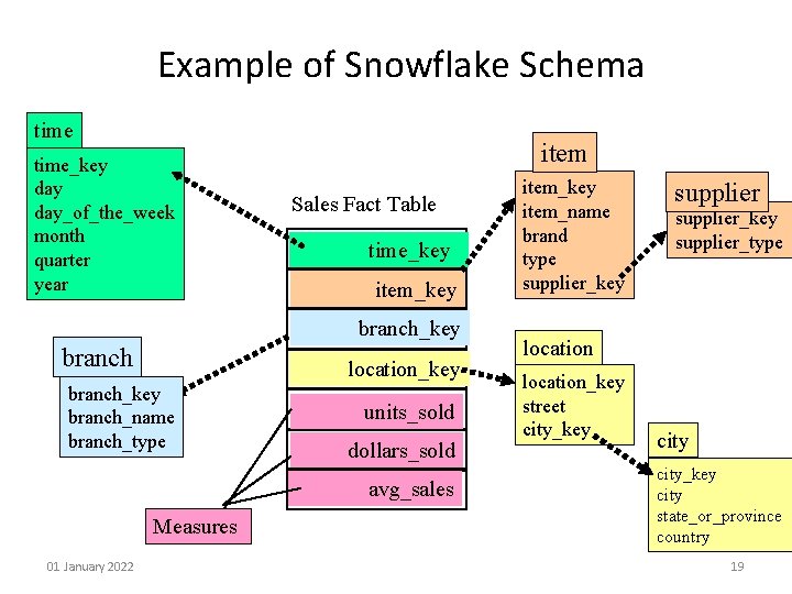
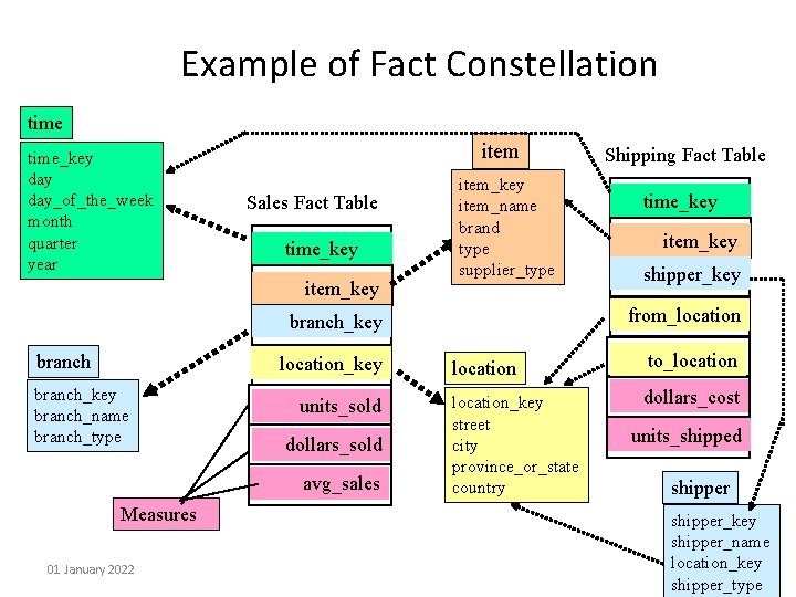
Conceptual Modeling of Data Warehouses • Modeling data warehouses: dimensions & measures – Star schema: A fact table in the middle connected to a set of dimension tables – Snowflake schema: A refinement of star schema where some dimensional hierarchy is normalized into a set of smaller dimension tables, forming a shape similar to snowflake – Fact constellations: Multiple fact tables share dimension tables, viewed as a collection of stars, therefore called galaxy schema or fact constellation 01 January 2022 14

Star Schemas • Data modeling technique used to map multidimensional decision support data into a relational database – Creates the near equivalent of a multidimensional database schema from the existing relational database – The schema was developed because existing relational modeling techniques, ER and normalization did not yield a database structure that served advanced data analysis requirements well • Yield an easily implemented model for multidimensional data analysis, while still preserving the relational structures on which the operational database is built • Has four components: facts, dimensions, attributes, and attribute hierarchies 01 January 2022 15

Star Schemas • Facts: numeric values that represent a specific business aspect or activity (sales figures). – The fact table contains facts that are linked through their dimensions – Metrics are facts computed or derived at run time • Dimensions: qualifying characteristics that provide additional perspectives to a fact (sales have product, location and time dimensions) – Dimensions are stored in a dimension table The Data Warehouse 16

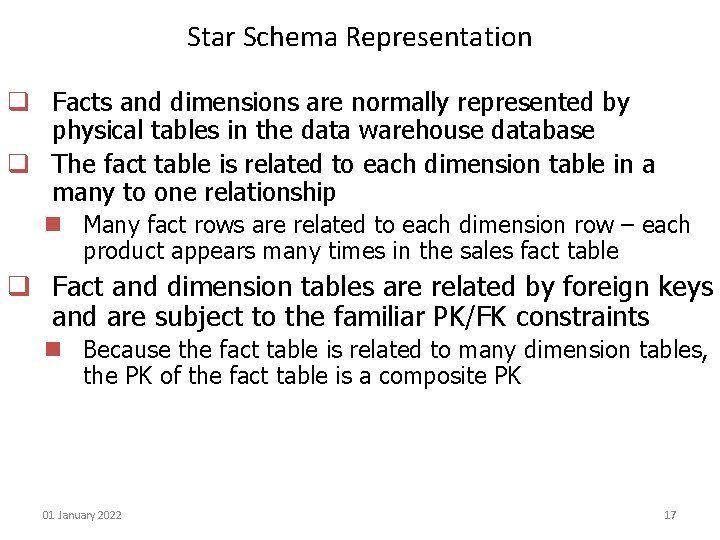
Star Schema Representation q Facts and dimensions are normally represented by physical tables in the data warehouse database q The fact table is related to each dimension table in a many to one relationship n Many fact rows are related to each dimension row – each product appears many times in the sales fact table q Fact and dimension tables are related by foreign keys and are subject to the familiar PK/FK constraints n Because the fact table is related to many dimension tables, the PK of the fact table is a composite PK 01 January 2022 17

Example of Star Schema time item time_key day_of_the_week month quarter year Sales Fact Table time_key item_key branch_key branch_name branch_type location_key units_sold dollars_sold avg_sales item_key item_name brand type supplier_type location_key street city state_or_province country Measures 01 January 2022 18

Example of Snowflake Schema time_key day_of_the_week month quarter year item Sales Fact Table time_key item_key branch location_key branch_name branch_type units_sold dollars_sold avg_sales Measures 01 January 2022 item_key item_name brand type supplier_key supplier_type location_key street city_key city state_or_province country 19

Example of Fact Constellation time_key day_of_the_week month quarter year item Sales Fact Table time_key item_key item_name brand type supplier_type location_key branch_name branch_type units_sold dollars_sold avg_sales Measures 01 January 2022 time_key item_key shipper_key from_location branch_key branch Shipping Fact Table location to_location_key street city province_or_state country dollars_cost units_shipped shipper_key shipper_name location_key 20 shipper_type

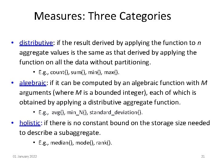
Measures: Three Categories • distributive: if the result derived by applying the function to n aggregate values is the same as that derived by applying the function on all the data without partitioning. • E. g. , count(), sum(), min(), max(). • algebraic: if it can be computed by an algebraic function with M arguments (where M is a bounded integer), each of which is obtained by applying a distributive aggregate function. • E. g. , avg(), min_N(), standard_deviation(). • holistic: if there is no constant bound on the storage size needed to describe a subaggregate. • E. g. , median(), mode(), rank(). 01 January 2022 21

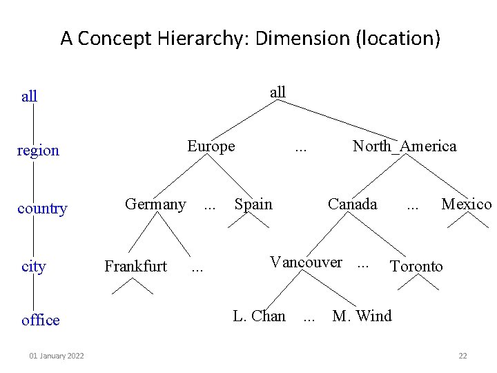
A Concept Hierarchy: Dimension (location) all Europe region country city office 01 January 2022 Germany Frankfurt . . Spain North_America Canada Vancouver. . . L. Chan . . . Mexico Toronto M. Wind 22

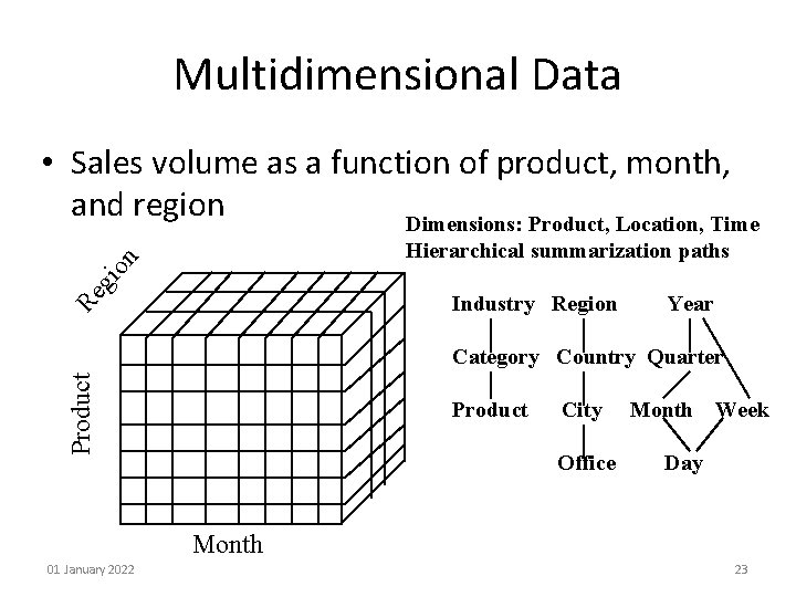
Multidimensional Data • Sales volume as a function of product, month, and region Dimensions: Product, Location, Time gi on Hierarchical summarization paths Re Industry Region Year Product Category Country Quarter Product City Office Month Week Day Month 01 January 2022 23

Cuboids Corresponding to the Cube all 0 -D(apex) cuboid product, date country product, country 1 -D cuboids date, country 2 -D cuboids product, date, country 01 January 2022 3 -D(base) cuboid 24

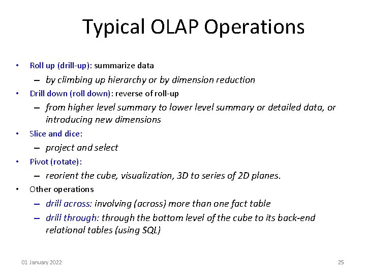
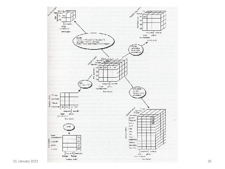
Typical OLAP Operations • Roll up (drill-up): summarize data – by climbing up hierarchy or by dimension reduction • Drill down (roll down): reverse of roll-up – from higher level summary to lower level summary or detailed data, or introducing new dimensions • Slice and dice: – project and select • Pivot (rotate): – reorient the cube, visualization, 3 D to series of 2 D planes. • Other operations – drill across: involving (across) more than one fact table – drill through: through the bottom level of the cube to its back-end relational tables (using SQL) 01 January 2022 25

01 January 2022 26

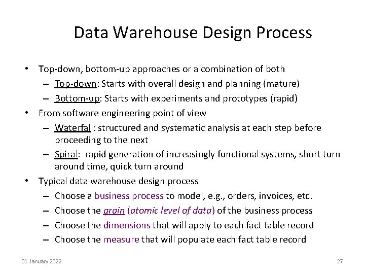
Data Warehouse Design Process • Top-down, bottom-up approaches or a combination of both – Top-down: Starts with overall design and planning (mature) – Bottom-up: Starts with experiments and prototypes (rapid) • From software engineering point of view – Waterfall: structured and systematic analysis at each step before proceeding to the next – Spiral: rapid generation of increasingly functional systems, short turn around time, quick turn around • Typical data warehouse design process – Choose a business process to model, e. g. , orders, invoices, etc. – Choose the grain (atomic level of data) of the business process – Choose the dimensions that will apply to each fact table record – Choose the measure that will populate each fact table record 01 January 2022 27

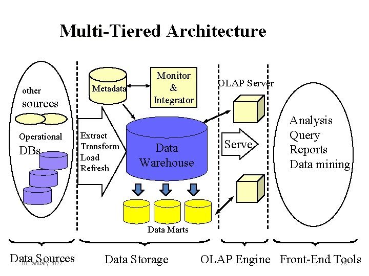
Multi-Tiered Architecture other Metadata sources Operational DBs Extract Transform Load Refresh Monitor & Integrator Data Warehouse OLAP Server Serve Analysis Query Reports Data mining Data Marts Data Sources 01 January 2022 Data Storage OLAP Engine Front-End Tools 28

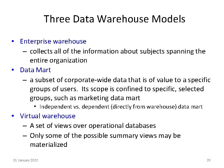
Three Data Warehouse Models • Enterprise warehouse – collects all of the information about subjects spanning the entire organization • Data Mart – a subset of corporate-wide data that is of value to a specific groups of users. Its scope is confined to specific, selected groups, such as marketing data mart • Independent vs. dependent (directly from warehouse) data mart • Virtual warehouse – A set of views over operational databases – Only some of the possible summary views may be materialized 01 January 2022 29

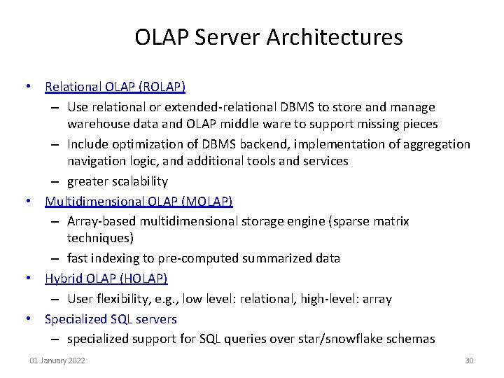
OLAP Server Architectures • Relational OLAP (ROLAP) – Use relational or extended-relational DBMS to store and manage warehouse data and OLAP middle ware to support missing pieces – Include optimization of DBMS backend, implementation of aggregation navigation logic, and additional tools and services – greater scalability • Multidimensional OLAP (MOLAP) – Array-based multidimensional storage engine (sparse matrix techniques) – fast indexing to pre-computed summarized data • Hybrid OLAP (HOLAP) – User flexibility, e. g. , low level: relational, high-level: array • Specialized SQL servers – specialized support for SQL queries over star/snowflake schemas 01 January 2022 30

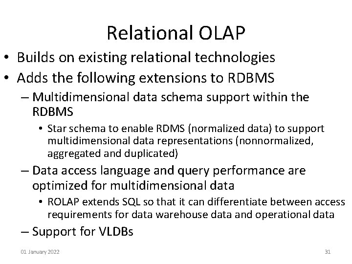
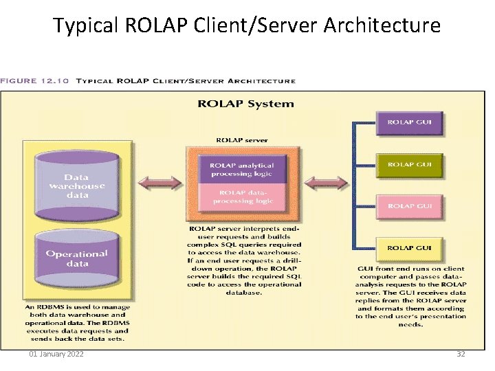
Relational OLAP • Builds on existing relational technologies • Adds the following extensions to RDBMS – Multidimensional data schema support within the RDBMS • Star schema to enable RDMS (normalized data) to support multidimensional data representations (nonnormalized, aggregated and duplicated) – Data access language and query performance are optimized for multidimensional data • ROLAP extends SQL so that it can differentiate between access requirements for data warehouse data and operational data – Support for VLDBs 01 January 2022 31

Typical ROLAP Client/Server Architecture 01 January 2022 32

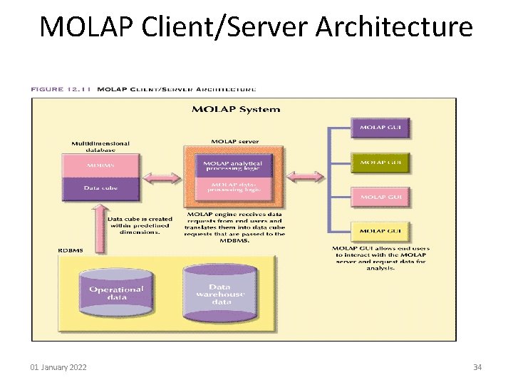
Multidimensional OLAP • MOLAP extends OLAP functionality to multidimensional DBMSs (MDBMSs) – An MDBMS stores data in matrix-like n-dimensional arrays – MDBMS end users visualize the stored data as a three-dimensional cube known as a data cube • They data cubes can grow to n-dimensions becoming hypercubes • Data cubes are created by extracting data from the operational databases or the data warehouse • They are pre-created and static and queried based on their dimensions e. g. , product, location and time for a cube for sales • To speed data access they are held in memory – cube cache 01 January 2022 33

MOLAP Client/Server Architecture 01 January 2022 34

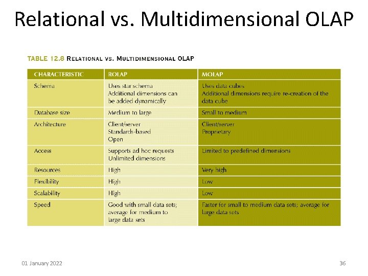
MDBMS • Because a cube is pre-defined, the addition of a new dimension requires that the entire data cube be recreated – a time consuming process – If this needs to be done often, the MDBMS loses some of its speed advantage over the RDBMS – MDBMS is best suited for small and medium data sets – Scalability is limited due to the restrictions on the size of the data cube to avoid lengthy data access times caused by having less memory available for the OS and application programs – Employ proprietary data storage techniques that require proprietary data access methods using a multidimensional query language – Most handle sparsity of the data cubes effectively to reduce processing overhead and resource requirements 01 January 2022 35

Relational vs. Multidimensional OLAP 01 January 2022 36

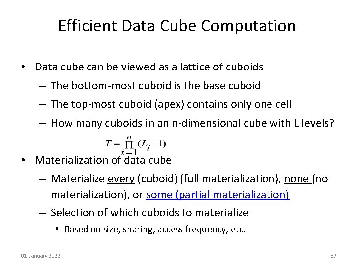
Efficient Data Cube Computation • Data cube can be viewed as a lattice of cuboids – The bottom-most cuboid is the base cuboid – The top-most cuboid (apex) contains only one cell – How many cuboids in an n-dimensional cube with L levels? • Materialization of data cube – Materialize every (cuboid) (full materialization), none (no materialization), or some (partial materialization) – Selection of which cuboids to materialize • Based on size, sharing, access frequency, etc. 01 January 2022 37

Materialized View “ Materialized views contains aggregate data (cuboids) derived from a fact table in order to minimize the query response time “ There are 3 kinds of materialization (Given a base cuboid ) 1. No Materialization – Precompute only the base cuboid • “ Slow response time ” 2. Full Materialization – Precompute all of the cuboids • “ Large storage space “ 3. Partial Materialization – Selectively compute a subset of the cuboids • “ Mix of the above “ 01 January 2022 38

Cube Computation: ROLAP-Based Method • ROLAP-based cubing algorithms – Sorting, hashing, and grouping operations are applied to the dimension attributes in order to reorder and cluster related tuples – Grouping is performed on some sub-aggregates as a “partial grouping step” – Aggregates may be computed from previously computed aggregates, rather than from the base fact table 01 January 2022 39

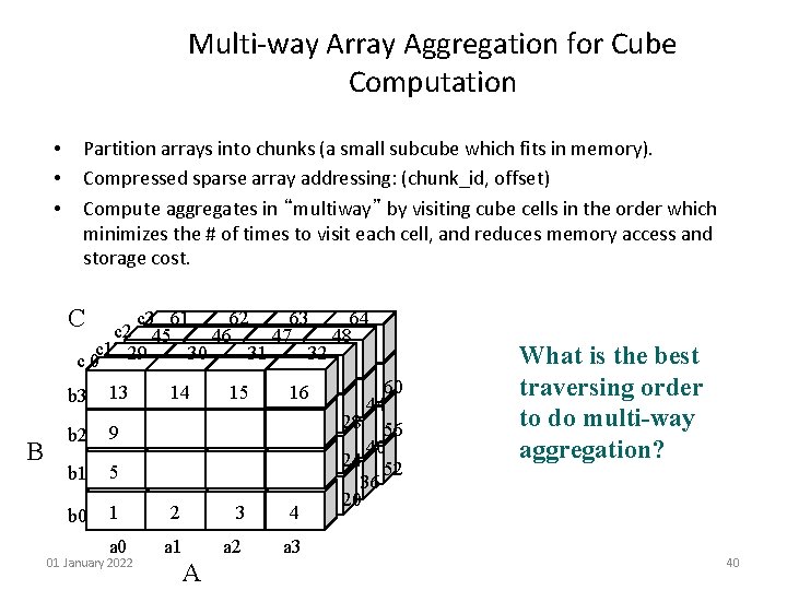
Multi-way Array Aggregation for Cube Computation • • • Partition arrays into chunks (a small subcube which fits in memory). Compressed sparse array addressing: (chunk_id, offset) Compute aggregates in “multiway” by visiting cube cells in the order which minimizes the # of times to visit each cell, and reduces memory access and storage cost. C c 3 61 62 63 64 c 2 45 46 47 48 c 1 29 30 31 32 c 0 B b 3 B 13 b 2 9 b 1 5 b 0 14 15 16 1 2 3 4 a 0 a 1 a 2 a 3 01 January 2022 A 60 44 28 56 40 24 52 36 20 What is the best traversing order to do multi-way aggregation? 40

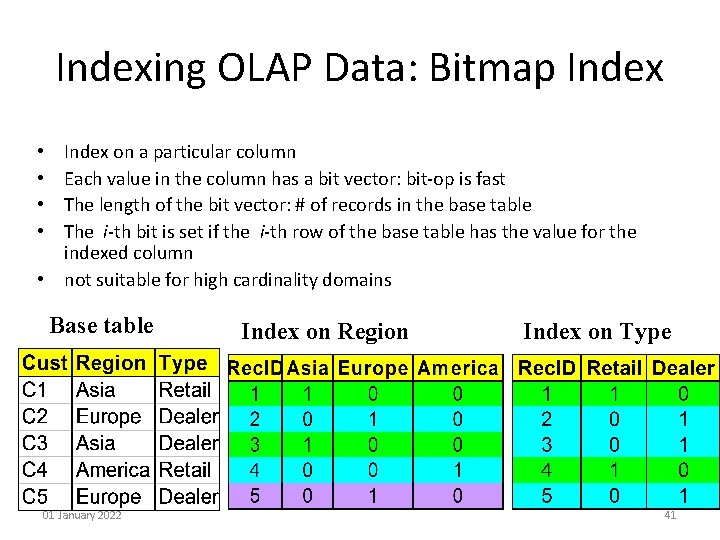
Indexing OLAP Data: Bitmap Index on a particular column Each value in the column has a bit vector: bit-op is fast The length of the bit vector: # of records in the base table The i-th bit is set if the i-th row of the base table has the value for the indexed column • not suitable for high cardinality domains • • Base table 01 January 2022 Index on Region Index on Type 41

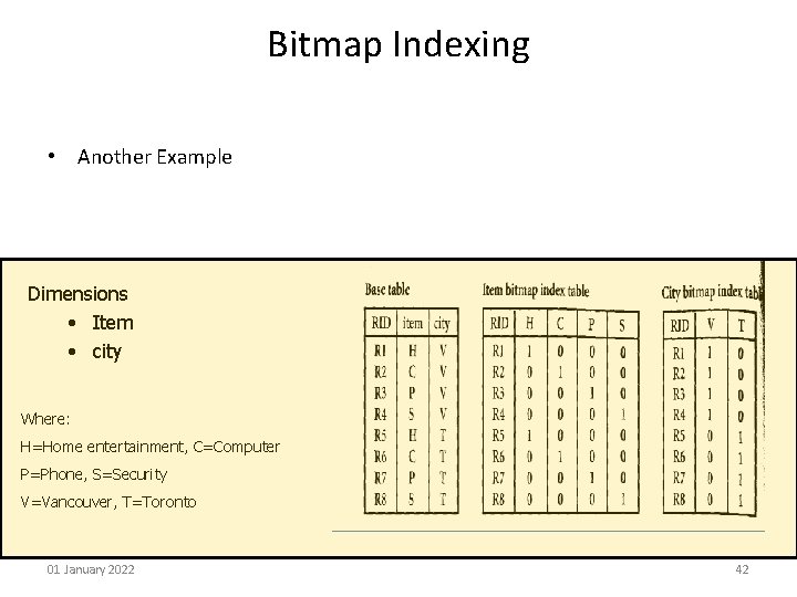
Bitmap Indexing • Another Example Dimensions • Item • city Where: H=Home entertainment, C=Computer P=Phone, S=Security V=Vancouver, T=Toronto 01 January 2022 42

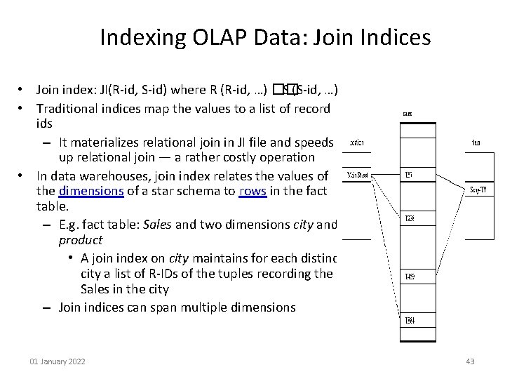
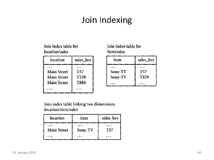
Indexing OLAP Data: Join Indices • Join index: JI(R-id, S-id) where R (R-id, …) �� S (S-id, …) • Traditional indices map the values to a list of record ids – It materializes relational join in JI file and speeds up relational join — a rather costly operation • In data warehouses, join index relates the values of the dimensions of a star schema to rows in the fact table. – E. g. fact table: Sales and two dimensions city and product • A join index on city maintains for each distinct city a list of R-IDs of the tuples recording the Sales in the city – Join indices can span multiple dimensions 01 January 2022 43

Join Indexing 01 January 2022 44

Efficient Processing of OLAP Queries • Determine which operations should be performed on the available cuboids: – transform drill, roll, etc. into corresponding SQL and/or OLAP operations, e. g, dice = selection + projection • Determine to which materialized cuboid(s) the relevant operations should be applied. • Exploring indexing structures and compressed vs. dense array structures in MOLAP 01 January 2022 45

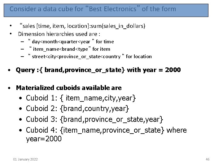
Consider a data cube for “Best Electronics” of the form • “sales [time, item, location]: sum(sales_in_dollars) • Dimension hierarchies used are : – “ day<month<quarter<year ” for time – “ item_name<brand<type” for item – “ street<city<province_or_state<country “ for location • Query : { brand, province_or_state} with year = 2000 • Materialized cuboids available are • • Cuboid 1: { item_name, city, year} Cuboid 2: {brand, country, year} Cuboid 3: {brand, province_or_state, year} Cuboid 4: {item_name, province_or_state} where year=2000 01 January 2022 46

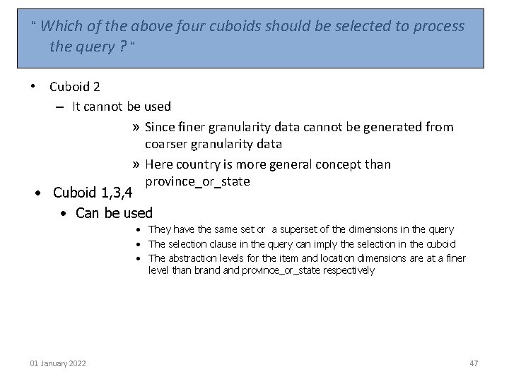
“ Which of the above four cuboids should be selected to process the query ? “ • Cuboid 2 – It cannot be used » Since finer granularity data cannot be generated from coarser granularity data » Here country is more general concept than province_or_state • Cuboid 1, 3, 4 • Can be used • They have the same set or a superset of the dimensions in the query • The selection clause in the query can imply the selection in the cuboid • The abstraction levels for the item and location dimensions are at a finer level than brand province_or_state respectively 01 January 2022 47

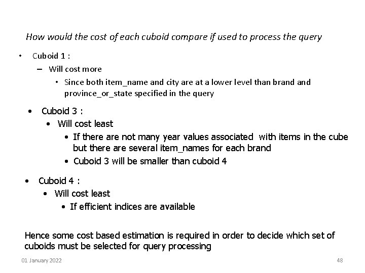
How would the cost of each cuboid compare if used to process the query Cuboid 1 : – Will cost more • Since both item_name and city are at a lower level than brand province_or_state specified in the query • • • Cuboid 3 : • Will cost least • If there are not many year values associated with items in the cube but there are several item_names for each brand • Cuboid 3 will be smaller than cuboid 4 Cuboid 4 : • Will cost least • If efficient indices are available Hence some cost based estimation is required in order to decide which set of cuboids must be selected for query processing 01 January 2022 48

Metadata Repository • Meta data is the data defining warehouse objects. It has the following kinds – Description of the structure of the warehouse • schema, view, dimensions, hierarchies, derived data defn, data mart locations and contents – Operational meta-data • data lineage (history of migrated data and transformation path), currency of data (active, archived, or purged), monitoring information (warehouse usage statistics, error reports, audit trails) – The algorithms used for summarization – The mapping from operational environment to the data warehouse – Data related to system performance • warehouse schema, view and derived data definitions – Business data • business terms and definitions, ownership of data, charging policies 01 January 2022 49

Data Warehouse Usage • Three kinds of data warehouse applications – Information processing • supports querying, basic statistical analysis, and reporting using crosstabs, tables, charts and graphs – Analytical processing • multidimensional analysis of data warehouse data • supports basic OLAP operations, slice-dice, drilling, pivoting – Data mining • knowledge discovery from hidden patterns • supports associations, constructing analytical models, performing classification and prediction, and presenting the mining results using visualization tools. • Differences among the three tasks 01 January 2022 50

From On-Line Analytical Processing to On Line Analytical Mining (OLAM) • Why online analytical mining? – High quality of data in data warehouses • DW contains integrated, consistent, cleaned data – Available information processing structure surrounding data warehouses • ODBC, OLEDB, Web accessing, service facilities, reporting and OLAP tools – OLAP-based exploratory data analysis • mining with drilling, dicing, pivoting, etc. – On-line selection of data mining functions • integration and swapping of multiple mining functions, algorithms, and tasks. 01 January 2022 51

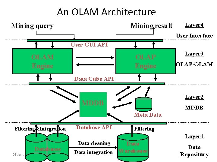
An OLAM Architecture Mining query Mining result Layer 4 User Interface User GUI API OLAM Engine OLAP Engine Layer 3 OLAP/OLAM Data Cube API Layer 2 MDDB Meta Data Filtering&Integration Database API Filtering Layer 1 Databases 01 January 2022 Data cleaning Data integration Warehouse Data 52 Repository

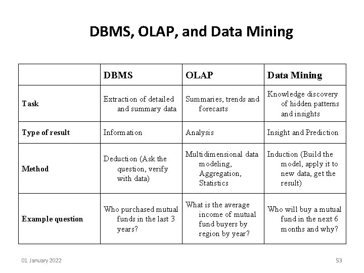
DBMS, OLAP, and Data Mining DBMS OLAP Data Mining Task Extraction of detailed and summary data Summaries, trends and forecasts Knowledge discovery of hidden patterns and insights Type of result Information Analysis Insight and Prediction Method Deduction (Ask the question, verify with data) Multidimensional data modeling, Aggregation, Statistics Induction (Build the model, apply it to new data, get the result) Example question Who purchased mutual funds in the last 3 years? What is the average income of mutual fund buyers by region by year? Who will buy a mutual fund in the next 6 months and why? 01 January 2022 53

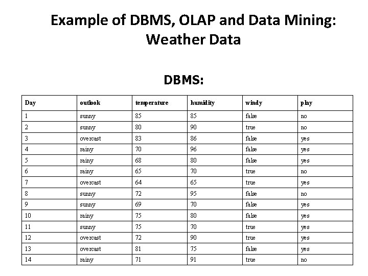
Example of DBMS, OLAP and Data Mining: Weather Data DBMS: Day outlook temperature humidity windy play 1 sunny 85 85 false no 2 sunny 80 90 true no 3 overcast 83 86 false yes 4 rainy 70 96 false yes 5 rainy 68 80 false yes 6 rainy 65 70 true no 7 overcast 64 65 true yes 8 sunny 72 95 false no 9 sunny 69 70 false yes 10 rainy 75 80 false yes 11 sunny 75 70 true yes 12 overcast 72 90 true yes 13 overcast 81 75 false yes 14 rainy 71 91 true no

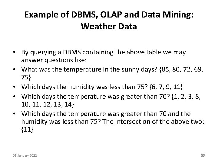
Example of DBMS, OLAP and Data Mining: Weather Data • By querying a DBMS containing the above table we may answer questions like: • What was the temperature in the sunny days? {85, 80, 72, 69, 75} • Which days the humidity was less than 75? {6, 7, 9, 11} • Which days the temperature was greater than 70? {1, 2, 3, 8, 10, 11, 12, 13, 14} • Which days the temperature was greater than 70 and the humidity was less than 75? The intersection of the above two: {11} 01 January 2022 55

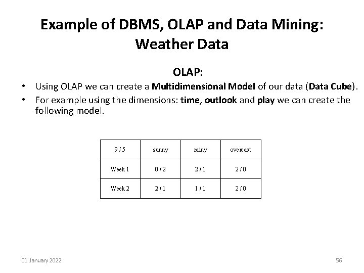
Example of DBMS, OLAP and Data Mining: Weather Data OLAP: • Using OLAP we can create a Multidimensional Model of our data (Data Cube). • For example using the dimensions: time, outlook and play we can create the following model. 01 January 2022 9/5 sunny rainy overcast Week 1 0/2 2/1 2/0 Week 2 2/1 1/1 2/0 56

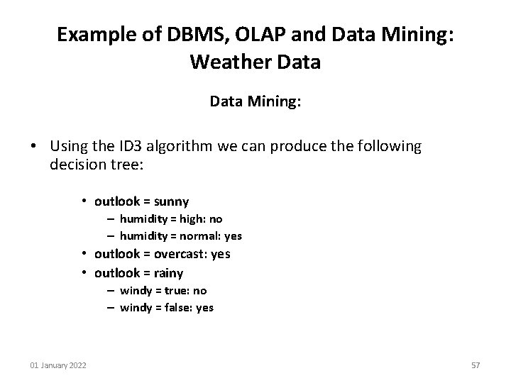
Example of DBMS, OLAP and Data Mining: Weather Data Mining: • Using the ID 3 algorithm we can produce the following decision tree: • outlook = sunny – humidity = high: no – humidity = normal: yes • outlook = overcast: yes • outlook = rainy – windy = true: no – windy = false: yes 01 January 2022 57

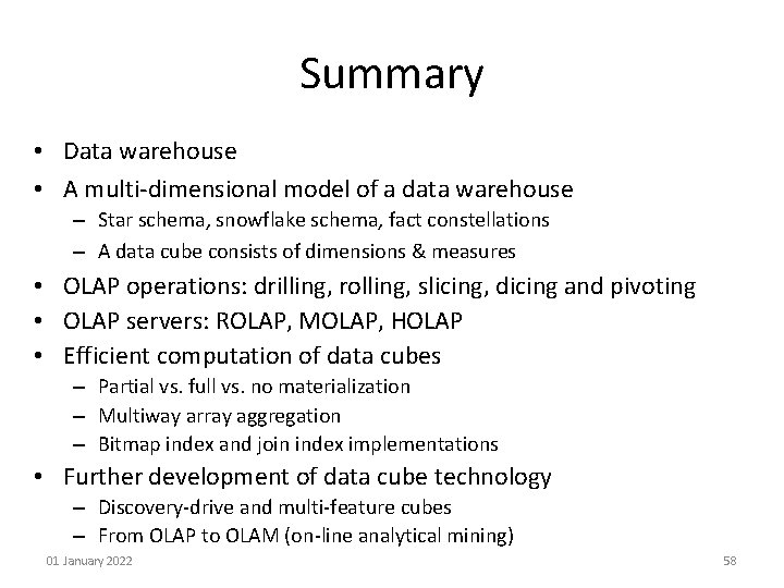
Summary • Data warehouse • A multi-dimensional model of a data warehouse – Star schema, snowflake schema, fact constellations – A data cube consists of dimensions & measures • OLAP operations: drilling, rolling, slicing, dicing and pivoting • OLAP servers: ROLAP, MOLAP, HOLAP • Efficient computation of data cubes – Partial vs. full vs. no materialization – Multiway array aggregation – Bitmap index and join index implementations • Further development of data cube technology – Discovery-drive and multi-feature cubes – From OLAP to OLAM (on-line analytical mining) 01 January 2022 58