Data Structures and Algorithms Queue Scheduling Msury Mahunnah

Data Structures and Algorithms Queue Scheduling Msury Mahunnah Department of Computer Science The Institute of Finance Management

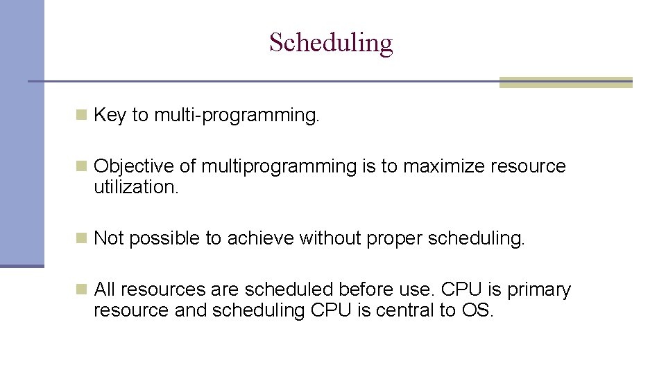
Scheduling n Key to multi-programming. n Objective of multiprogramming is to maximize resource utilization. n Not possible to achieve without proper scheduling. n All resources are scheduled before use. CPU is primary resource and scheduling CPU is central to OS.

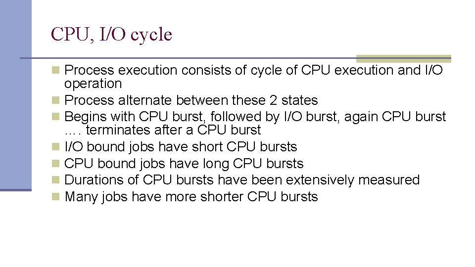
CPU, I/O cycle n Process execution consists of cycle of CPU execution and I/O operation n Process alternate between these 2 states n Begins with CPU burst, followed by I/O burst, again CPU burst …. terminates after a CPU burst n I/O bound jobs have short CPU bursts n CPU bound jobs have long CPU bursts n Durations of CPU bursts have been extensively measured n Many jobs have more shorter CPU bursts

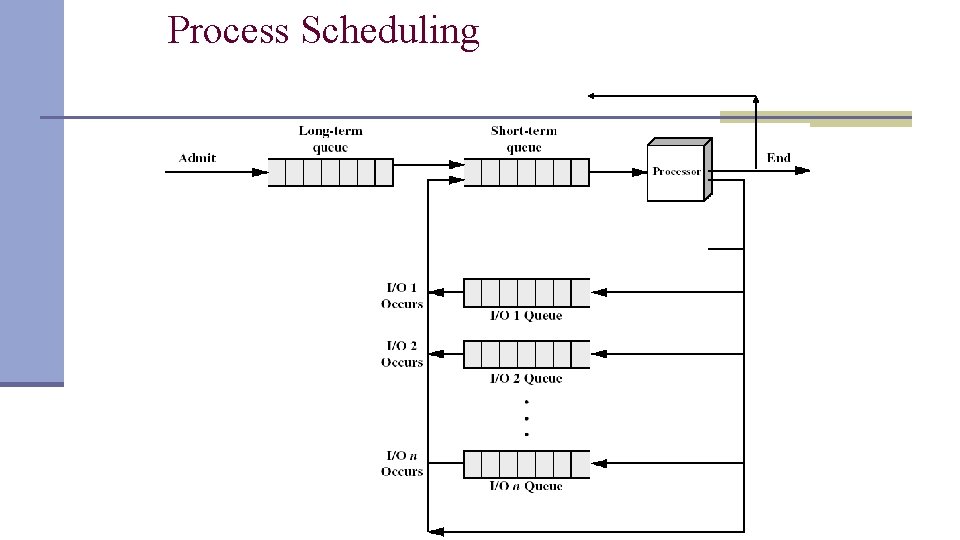
Process Scheduling

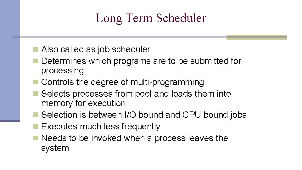
Long Term Scheduler n Also called as job scheduler n Determines which programs are to be submitted for processing n Controls the degree of multi-programming n Selects processes from pool and loads them into memory for execution n Selection is between I/O bound and CPU bound jobs n Executes much less frequently n Needs to be invoked when a process leaves the system

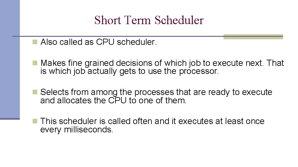
Short Term Scheduler n Also called as CPU scheduler. n Makes fine grained decisions of which job to execute next. That is which job actually gets to use the processor. n Selects from among the processes that are ready to execute and allocates the CPU to one of them. n This scheduler is called often and it executes at least once every milliseconds.

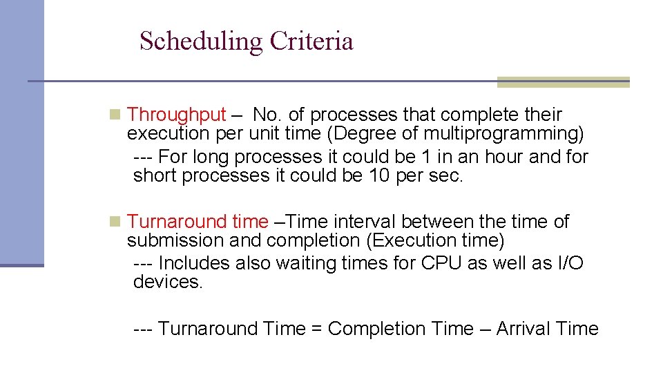
Scheduling Criteria n Throughput – No. of processes that complete their execution per unit time (Degree of multiprogramming) --- For long processes it could be 1 in an hour and for short processes it could be 10 per sec. n Turnaround time –Time interval between the time of submission and completion (Execution time) --- Includes also waiting times for CPU as well as I/O devices. --- Turnaround Time = Completion Time – Arrival Time

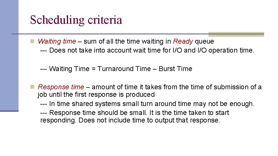
Scheduling criteria n Waiting time – sum of all the time waiting in Ready queue --- Does not take into account wait time for I/O and I/O operation time. --- Waiting Time = Turnaround Time – Burst Time n Response time – amount of time it takes from the time of submission of a job until the first response is produced --- In time shared systems small turn around time may not be enough. --- Response time should be small. It is the time taken to start responding. Does not include time to output that response.

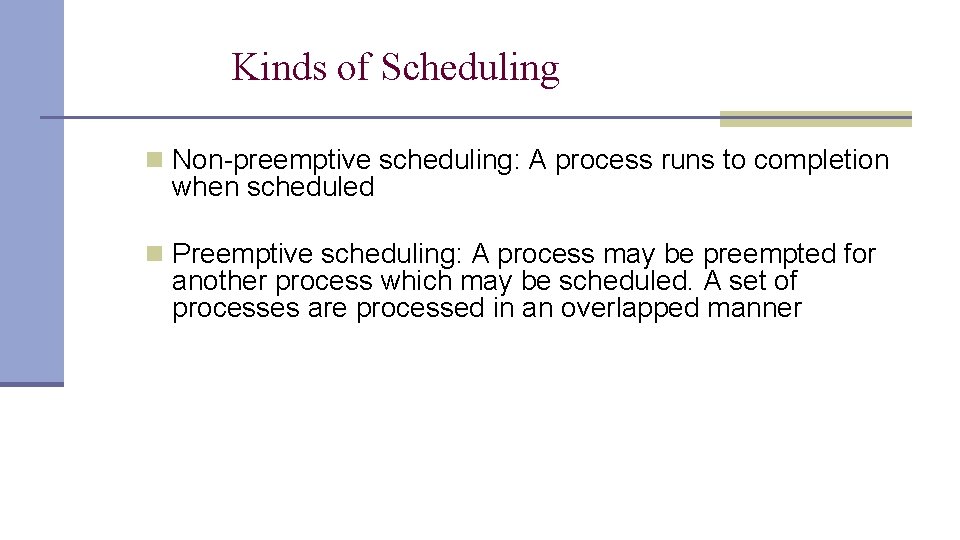
Kinds of Scheduling n Non-preemptive scheduling: A process runs to completion when scheduled n Preemptive scheduling: A process may be preempted for another process which may be scheduled. A set of processes are processed in an overlapped manner

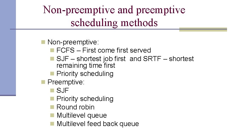
Non-preemptive and preemptive scheduling methods n Non-preemptive: n FCFS – First come first served n SJF – shortest job first and SRTF – shortest remaining time first n Priority scheduling n Preemptive: n SJF n Priority scheduling n Round robin n Multilevel queue n Multilevel feed back queue

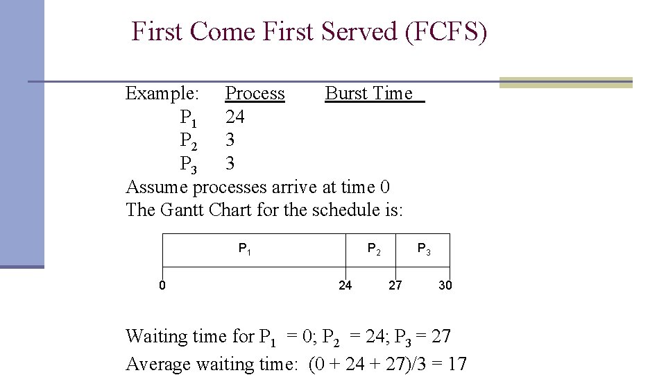
First Come First Served (FCFS) Example: Process Burst Time P 1 24 P 2 3 P 3 3 Assume processes arrive at time 0 The Gantt Chart for the schedule is: P 1 0 P 2 24 P 3 27 30 Waiting time for P 1 = 0; P 2 = 24; P 3 = 27 Average waiting time: (0 + 24 + 27)/3 = 17

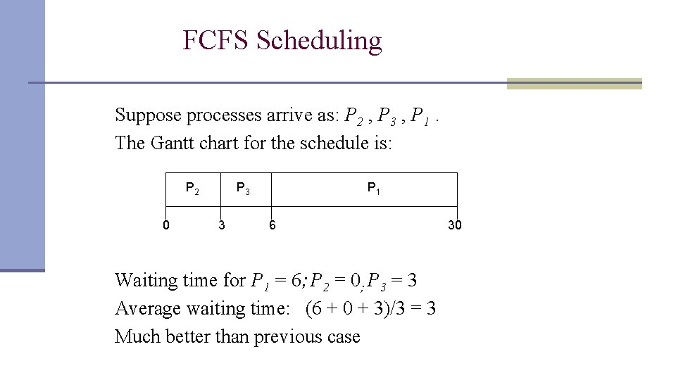
FCFS Scheduling Suppose processes arrive as: P 2 , P 3 , P 1. The Gantt chart for the schedule is: P 2 0 P 3 3 P 1 6 Waiting time for P 1 = 6; P 2 = 0; P 3 = 3 Average waiting time: (6 + 0 + 3)/3 = 3 Much better than previous case 30

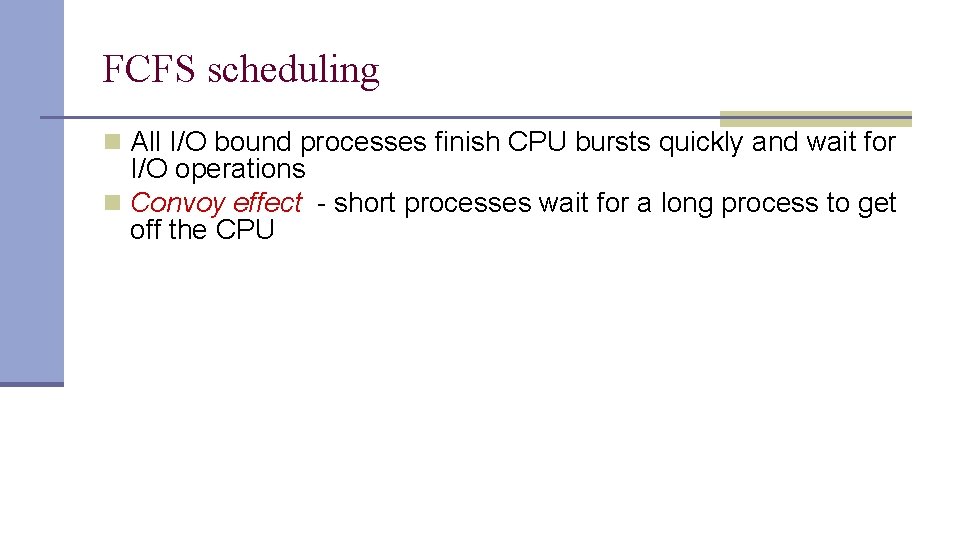
FCFS scheduling n All I/O bound processes finish CPU bursts quickly and wait for I/O operations n Convoy effect - short processes wait for a long process to get off the CPU

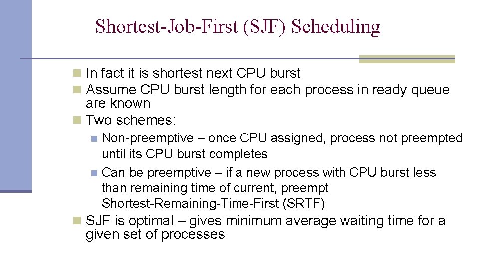
Shortest-Job-First (SJF) Scheduling n In fact it is shortest next CPU burst n Assume CPU burst length for each process in ready queue are known n Two schemes: Non-preemptive – once CPU assigned, process not preempted until its CPU burst completes n Can be preemptive – if a new process with CPU burst less than remaining time of current, preempt Shortest-Remaining-Time-First (SRTF) n n SJF is optimal – gives minimum average waiting time for a given set of processes

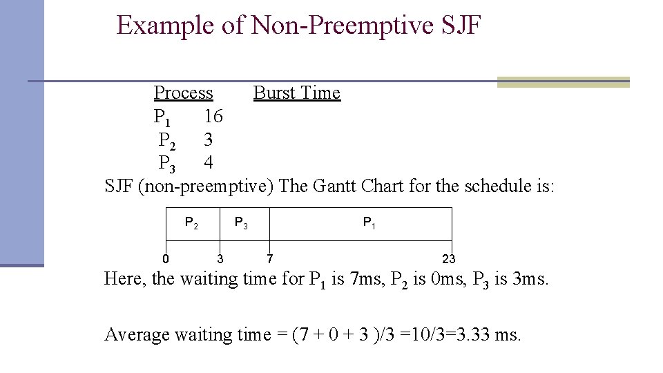
Example of Non-Preemptive SJF Process Burst Time P 1 16 P 2 3 P 3 4 SJF (non-preemptive) The Gantt Chart for the schedule is: P 2 0 P 3 3 P 1 7 23 Here, the waiting time for P 1 is 7 ms, P 2 is 0 ms, P 3 is 3 ms. Average waiting time = (7 + 0 + 3 )/3 =10/3=3. 33 ms.

Example of Preemptive SJF Process Arrival time Burst Time P 1 0 8 P 2 1 4 P 3 2 9 P 4 3 5 SJF (preemptive) The Gantt Chart for the schedule is: p 1 0 p 2 1 p 4 5 p 1 10 p 3 17 19 Average waiting time = (10 -1) +(17 -2)+(5 -3)/4 = 26/4 =6. 5 ms.

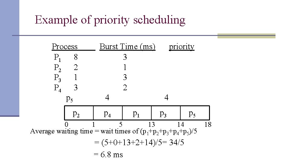
Example of priority scheduling Process P 1 8 P 2 2 P 3 1 P 4 3 p 5 p 2 Burst Time (ms) 3 1 3 2 4 p 1 priority 4 p 3 p 5 0 1 5 13 14 18 Average waiting time = wait times of (p 1+p 2+p 3+p 4+p 5)/5 = (5+0+13+2+14)/5= 34/5 = 6. 8 ms