CSE 421 Algorithms Richard Anderson Lecture 15 Fast

CSE 421 Algorithms Richard Anderson Lecture 15 Fast Fourier Transform

FFT, Convolution and Polynomial Multiplication • FFT: O(n log n) algorithm – Evaluate a polynomial of degree n at n points in O(n log n) time • Polynomial Multiplication: O(n log n) time

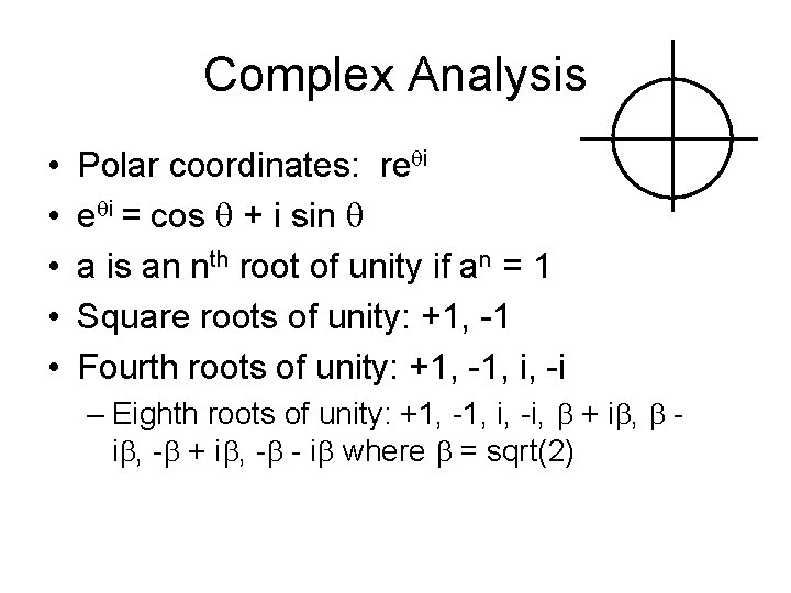
Complex Analysis • • • Polar coordinates: reqi = cos q + i sin q a is an nth root of unity if an = 1 Square roots of unity: +1, -1 Fourth roots of unity: +1, -1, i, -i – Eighth roots of unity: +1, -1, i, -i, b + ib, b ib, -b + ib, -b - ib where b = sqrt(2)

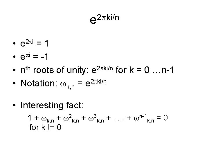
e 2 pki/n • • e 2 pi = 1 epi = -1 nth roots of unity: e 2 pki/n for k = 0 …n-1 Notation: wk, n = e 2 pki/n • Interesting fact: 1 + wk, n + w 2 k, n + w 3 k, n +. . . + wn-1 k, n = 0 for k != 0

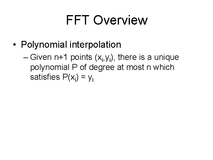
FFT Overview • Polynomial interpolation – Given n+1 points (xi, yi), there is a unique polynomial P of degree at most n which satisfies P(xi) = yi

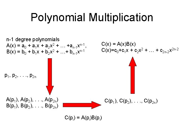
Polynomial Multiplication n-1 degree polynomials A(x) = a 0 + a 1 x + a 2 x 2 + … +an-1 xn-1, B(x) = b 0 + b 1 x + b 2 x 2 + …+ bn-1 xn-1 C(x) = A(x)B(x) C(x)=c 0+c 1 x + c 2 x 2 + … + c 2 n-2 x 2 n-2 p 1, p 2, . . . , p 2 n A(p 1), A(p 2), . . . , A(p 2 n) B(p 1), B(p 2), . . . , B(p 2 n) C(p 1), C(p 2), . . . , C(p 2 n) C(pi) = A(pi)B(pi)

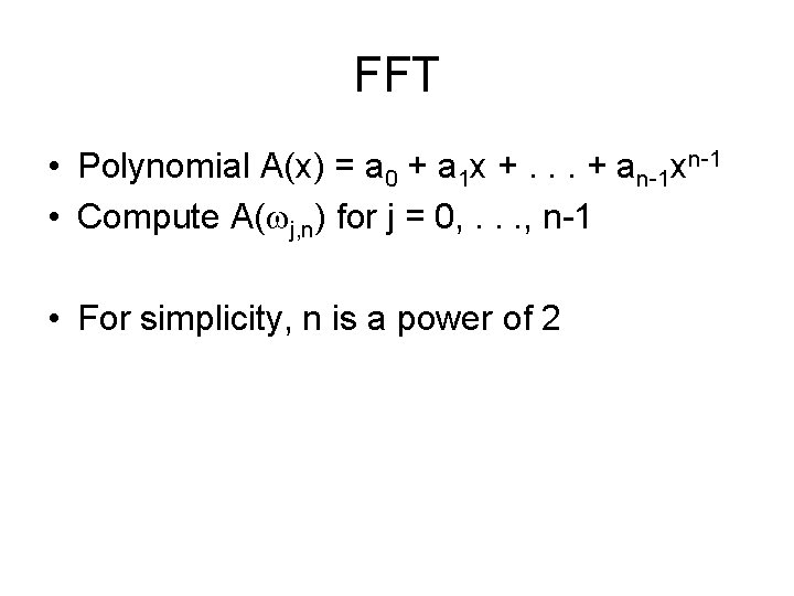
FFT • Polynomial A(x) = a 0 + a 1 x +. . . + an-1 xn-1 • Compute A(wj, n) for j = 0, . . . , n-1 • For simplicity, n is a power of 2

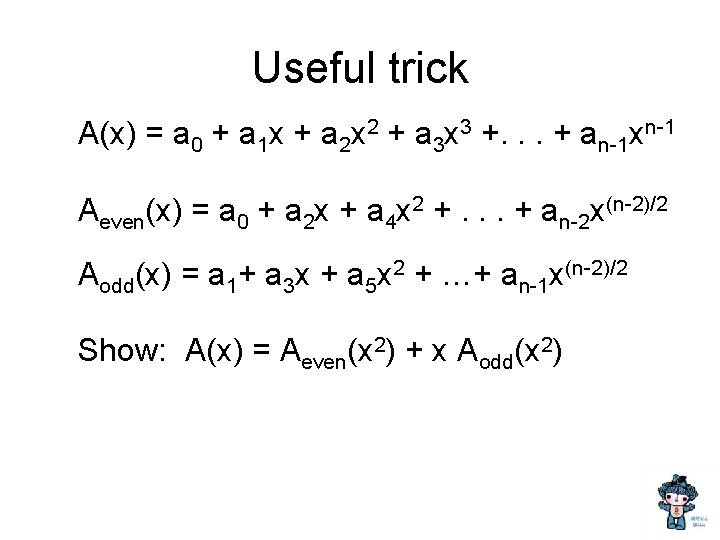
Useful trick A(x) = a 0 + a 1 x + a 2 x 2 + a 3 x 3 +. . . + an-1 xn-1 Aeven(x) = a 0 + a 2 x + a 4 x 2 +. . . + an-2 x(n-2)/2 Aodd(x) = a 1+ a 3 x + a 5 x 2 + …+ an-1 x(n-2)/2 Show: A(x) = Aeven(x 2) + x Aodd(x 2)

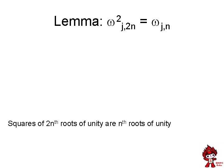
Lemma: w 2 j, 2 n = wj, n Squares of 2 nth roots of unity are nth roots of unity

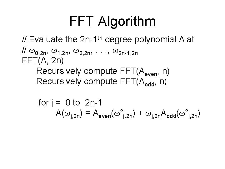
FFT Algorithm // Evaluate the 2 n-1 th degree polynomial A at // w 0, 2 n, w 1, 2 n, w 2, 2 n, . . . , w 2 n-1, 2 n FFT(A, 2 n) Recursively compute FFT(Aeven, n) Recursively compute FFT(Aodd, n) for j = 0 to 2 n-1 A(wj, 2 n) = Aeven(w 2 j, 2 n) + wj, 2 n. Aodd(w 2 j, 2 n)

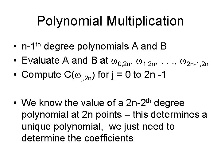
Polynomial Multiplication • n-1 th degree polynomials A and B • Evaluate A and B at w 0, 2 n, w 1, 2 n, . . . , w 2 n-1, 2 n • Compute C(wj, 2 n) for j = 0 to 2 n -1 • We know the value of a 2 n-2 th degree polynomial at 2 n points – this determines a unique polynomial, we just need to determine the coefficients

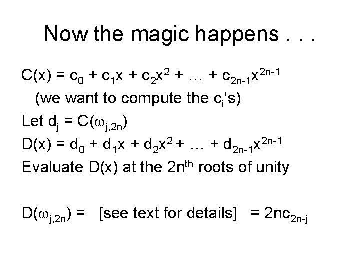
Now the magic happens. . . C(x) = c 0 + c 1 x + c 2 x 2 + … + c 2 n-1 x 2 n-1 (we want to compute the ci’s) Let dj = C(wj, 2 n) D(x) = d 0 + d 1 x + d 2 x 2 + … + d 2 n-1 x 2 n-1 Evaluate D(x) at the 2 nth roots of unity D(wj, 2 n) = [see text for details] = 2 nc 2 n-j

Polynomial Interpolation • Build polynomial from the values of C at the 2 nth roots of unity • Evaluate this polynomial at the 2 nth roots of unity

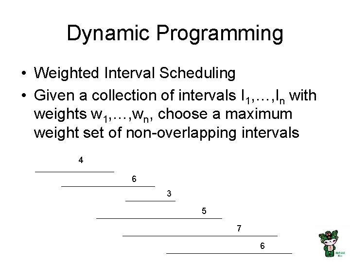
Dynamic Programming • Weighted Interval Scheduling • Given a collection of intervals I 1, …, In with weights w 1, …, wn, choose a maximum weight set of non-overlapping intervals 4 6 3 5 7 6

Recursive Algorithm Intervals sorted by finish time p[i] is the index of the last interval which finishes before i starts 1 2 3 4 5 6 7 8

Optimality Condition • Opt[j] is the maximum weight independent set of intervals I 1, I 2, . . . , Ij

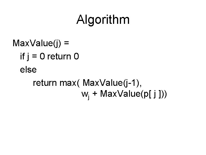
Algorithm Max. Value(j) = if j = 0 return 0 else return max( Max. Value(j-1), wj + Max. Value(p[ j ]))

Run time • What is the worst case run time of Max. Value • Design a worst case input

A better algorithm M[ j ] initialized to -1 before the first recursive call for all j Max. Value(j) = if j = 0 return 0; else if M[ j ] != -1 return M[ j ]; else M[ j ] = max(Max. Value(j-1), wj + Max. Value(p[ j ])); return M[ j ];