CSE 416 DIGITAL CONTROL Lecture 04 TimeResponse Characteristics

CSE 416: DIGITAL CONTROL Lecture 04: Time-Response Characteristics and Stability Dr. Ahmed Mahmoud, 16/11/2020

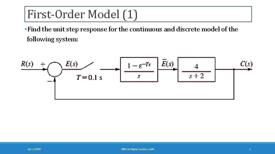
First-Order Model (1) • Find the unit step response for the continuous and discrete model of the following system: 16/11/2020 CSE 416: Digital Control, Lec 04 2

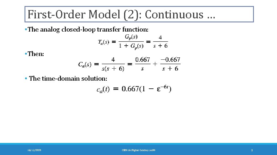
First-Order Model (2): Continuous … • The analog closed-loop transfer function: • The time-domain solution: 16/11/2020 CSE 416: Digital Control, Lec 04 3

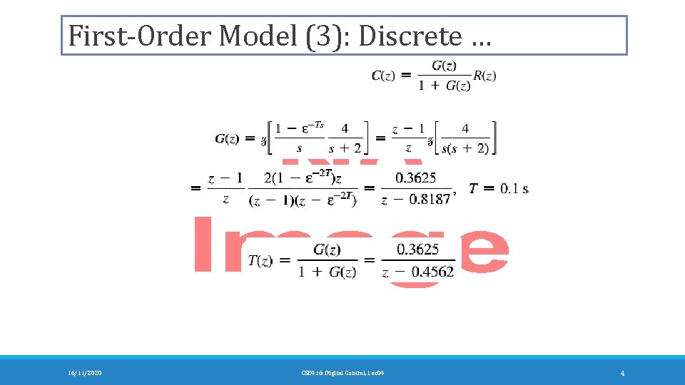
First-Order Model (3): Discrete … 16/11/2020 CSE 416: Digital Control, Lec 04 4

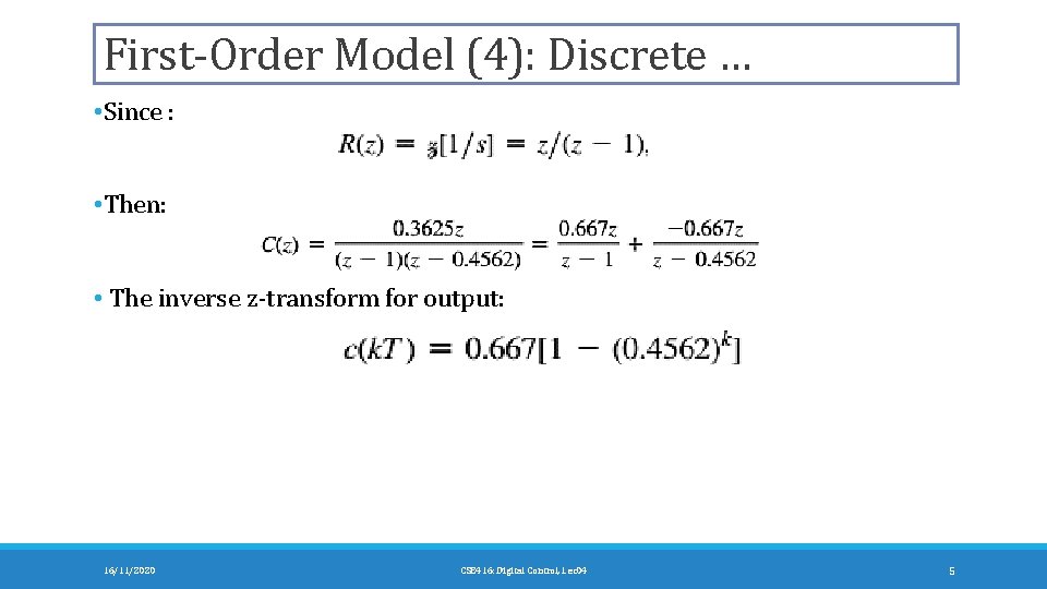
First-Order Model (4): Discrete … • Since : • Then: • The inverse z-transform for output: 16/11/2020 CSE 416: Digital Control, Lec 04 5

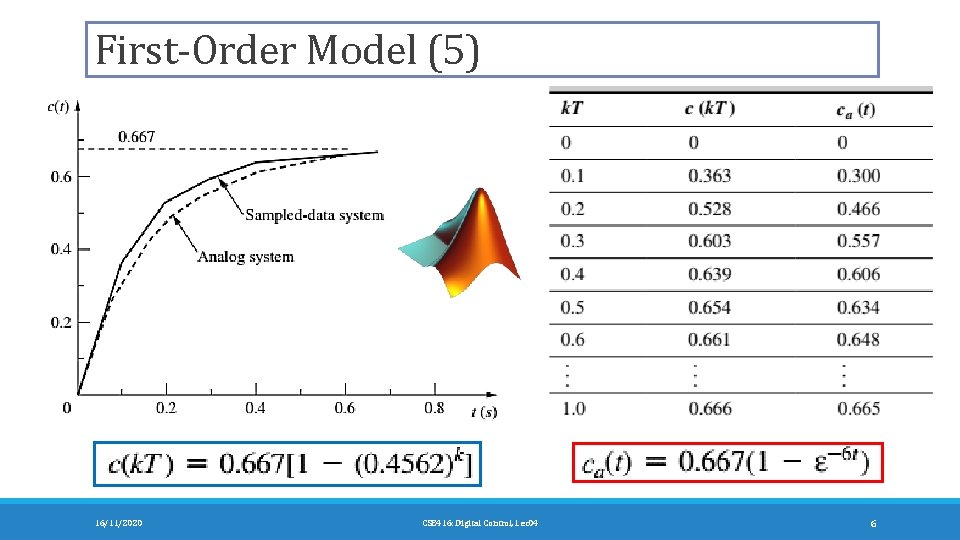
First-Order Model (5) 16/11/2020 CSE 416: Digital Control, Lec 04 6

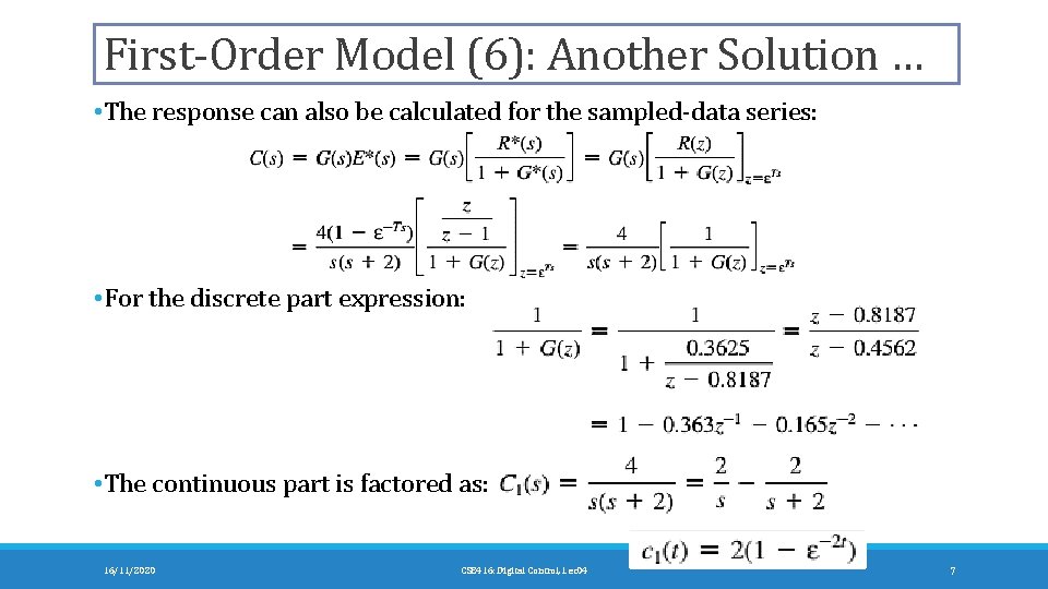
First-Order Model (6): Another Solution … • The response can also be calculated for the sampled-data series: • For the discrete part expression: • The continuous part is factored as: 16/11/2020 CSE 416: Digital Control, Lec 04 7

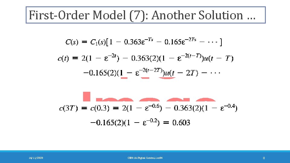
First-Order Model (7): Another Solution … 16/11/2020 CSE 416: Digital Control, Lec 04 8

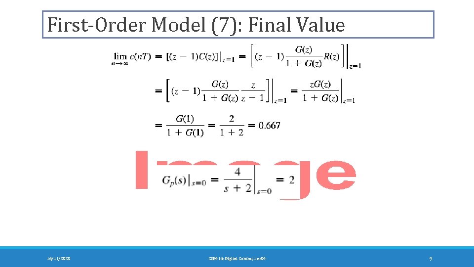
First-Order Model (7): Final Value 16/11/2020 CSE 416: Digital Control, Lec 04 9

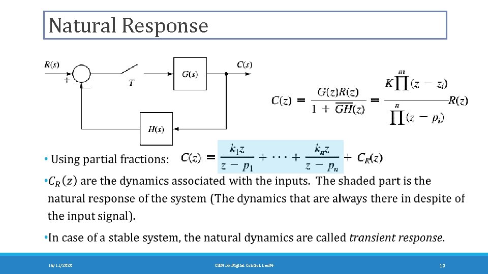
Natural Response 16/11/2020 CSE 416: Digital Control, Lec 04 10

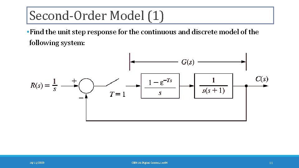
Second-Order Model (1) • Find the unit step response for the continuous and discrete model of the following system: 16/11/2020 CSE 416: Digital Control, Lec 04 11

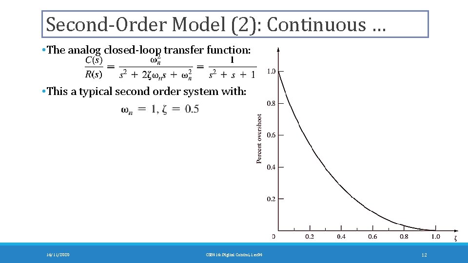
Second-Order Model (2): Continuous … • The analog closed-loop transfer function: • This a typical second order system with: 16/11/2020 CSE 416: Digital Control, Lec 04 12

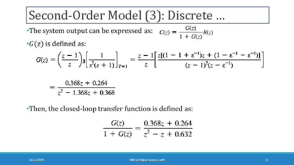
Second-Order Model (3): Discrete … 16/11/2020 CSE 416: Digital Control, Lec 04 13

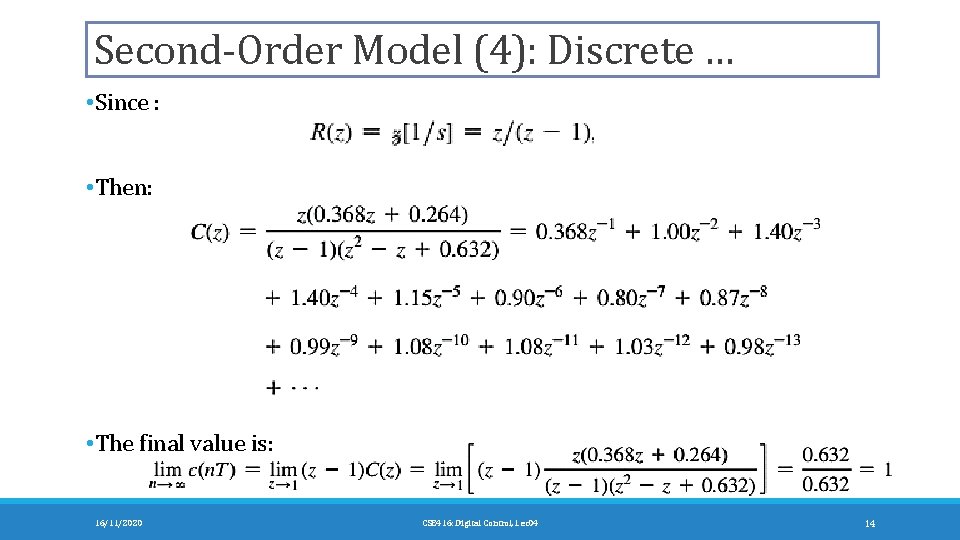
Second-Order Model (4): Discrete … • Since : • Then: • The final value is: 16/11/2020 CSE 416: Digital Control, Lec 04 14

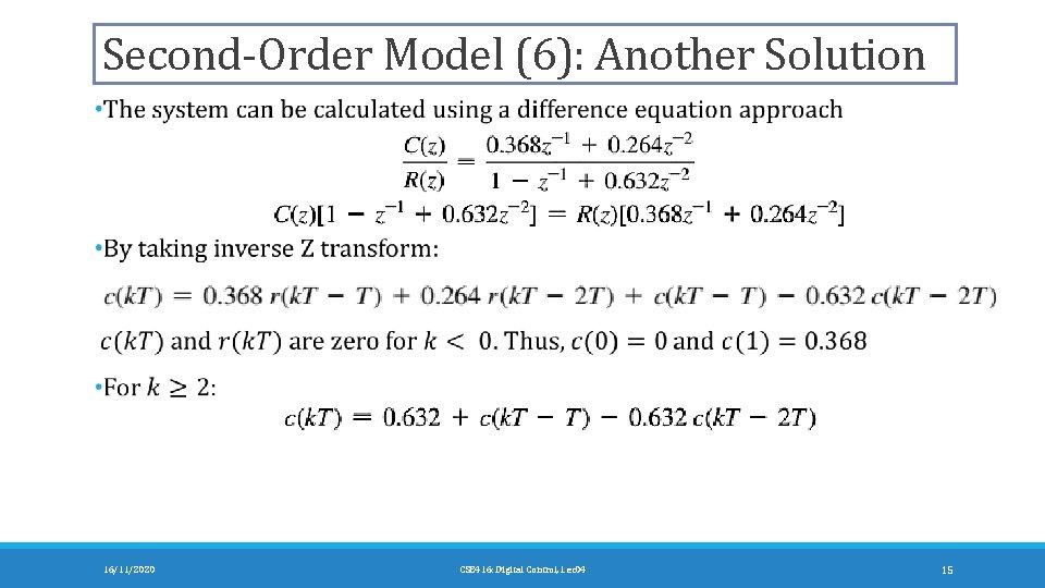
Second-Order Model (6): Another Solution 16/11/2020 CSE 416: Digital Control, Lec 04 15

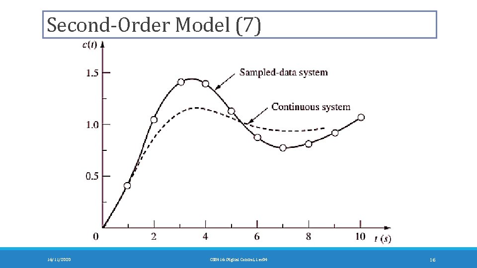
Second-Order Model (7) 16/11/2020 CSE 416: Digital Control, Lec 04 16

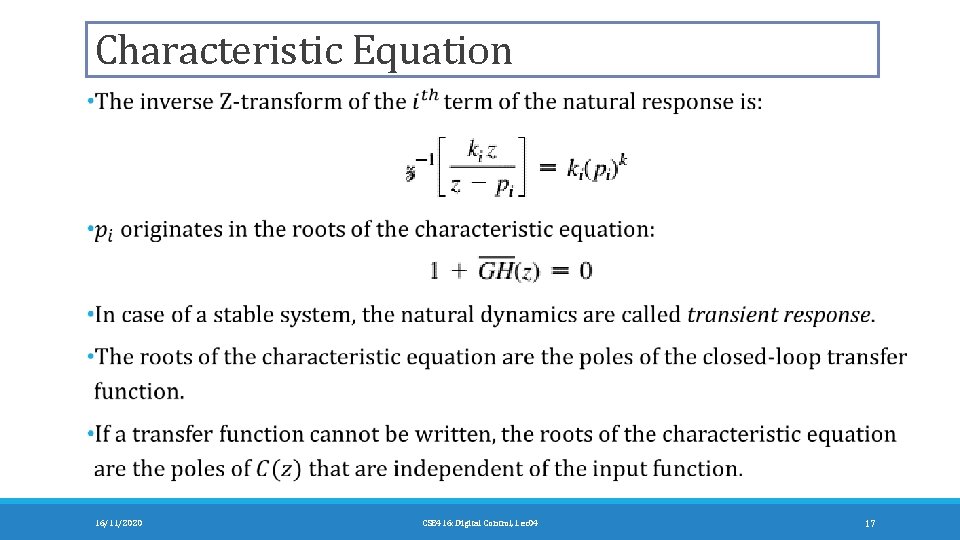
Characteristic Equation 16/11/2020 CSE 416: Digital Control, Lec 04 17

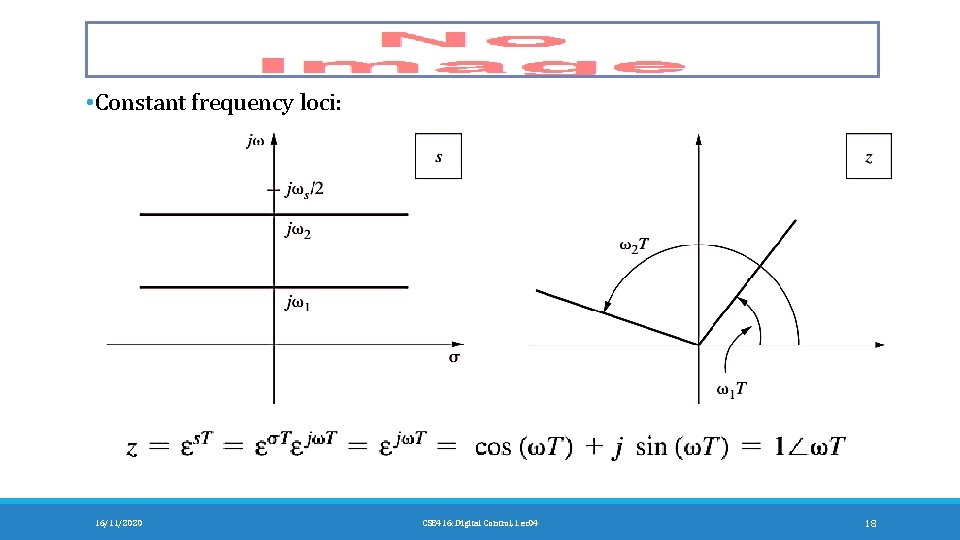
• Constant frequency loci: 16/11/2020 CSE 416: Digital Control, Lec 04 18

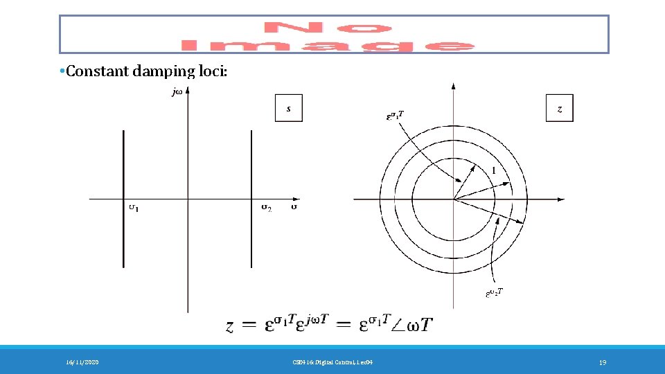
• Constant damping loci: 16/11/2020 CSE 416: Digital Control, Lec 04 19

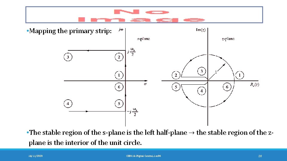
• Mapping the primary strip: • The stable region of the s-plane is the left half-plane → the stable region of the zplane is the interior of the unit circle. 16/11/2020 CSE 416: Digital Control, Lec 04 20

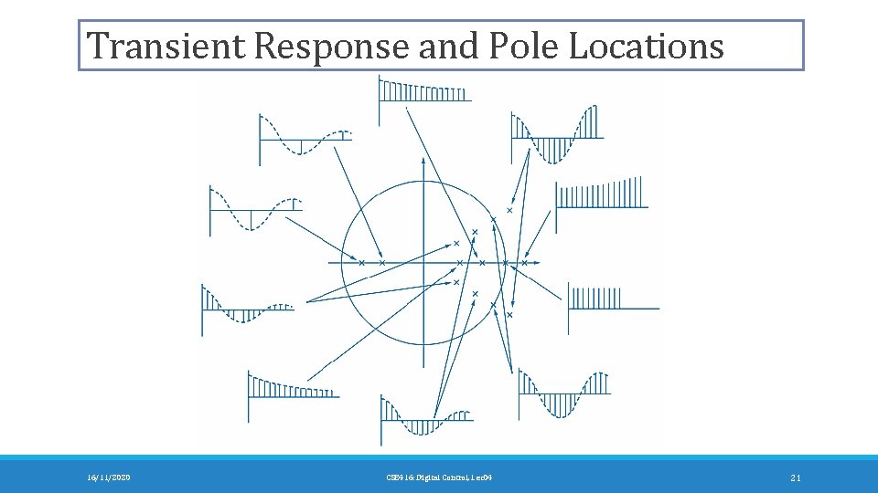
Transient Response and Pole Locations 16/11/2020 CSE 416: Digital Control, Lec 04 21

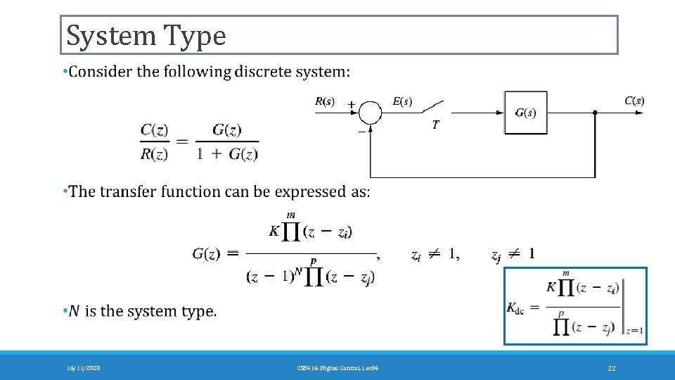
System Type 16/11/2020 CSE 416: Digital Control, Lec 04 22

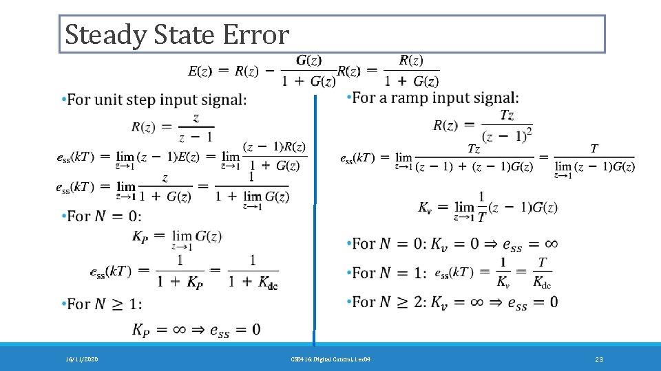
Steady State Error 16/11/2020 CSE 416: Digital Control, Lec 04 23

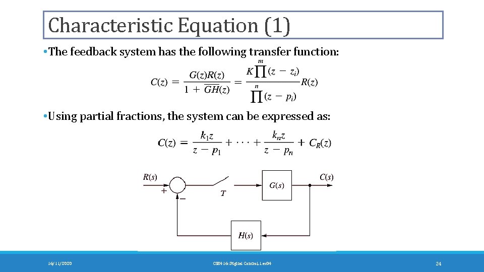
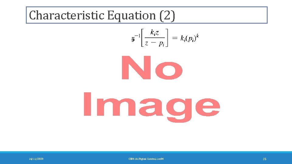
Characteristic Equation (1) • The feedback system has the following transfer function: • Using partial fractions, the system can be expressed as: 16/11/2020 CSE 416: Digital Control, Lec 04 24

Characteristic Equation (2) 16/11/2020 CSE 416: Digital Control, Lec 04 25

Stability for Discrete-time Systems • Many analysis and design techniques for continuous-time LTI systems, such as the Routh–Hurwitz criterion and Bode techniques, are based on the property that in the s-plane the stability boundary is the imaginary axis. • These techniques cannot be applied to LTI discrete-time systems in the z-plane since the stability boundary is the unit circle. • Either: 1. Transform the discrete-time system back to continuous system (Bilinear transform). 2. Use tools for discrete-time systems (Jury’s test). 16/11/2020 CSE 416: Digital Control, Lec 04 26

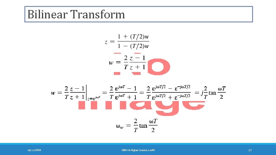
Bilinear Transform 16/11/2020 CSE 416: Digital Control, Lec 04 27

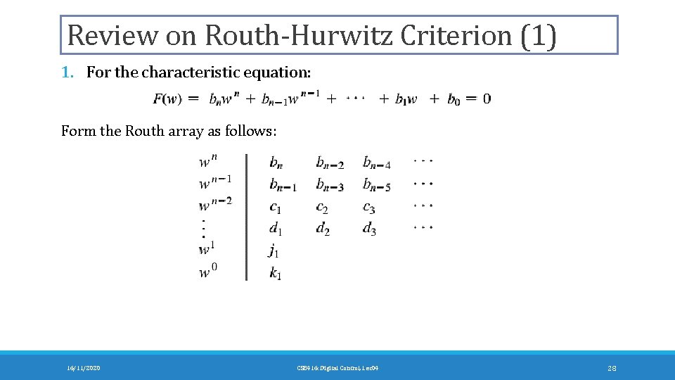
Review on Routh-Hurwitz Criterion (1) 1. For the characteristic equation: Form the Routh array as follows: 16/11/2020 CSE 416: Digital Control, Lec 04 28

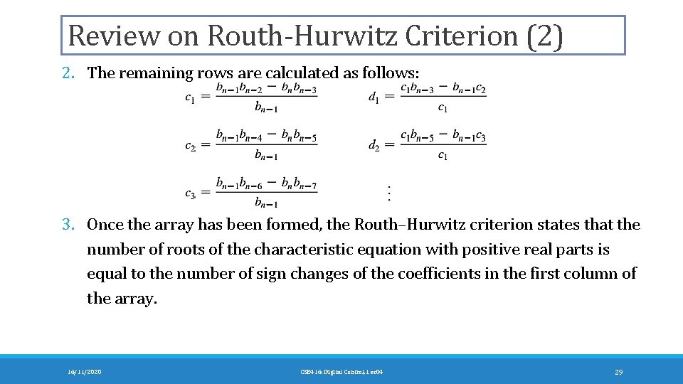
Review on Routh-Hurwitz Criterion (2) 2. The remaining rows are calculated as follows: 3. Once the array has been formed, the Routh–Hurwitz criterion states that the number of roots of the characteristic equation with positive real parts is equal to the number of sign changes of the coefficients in the first column of the array. 16/11/2020 CSE 416: Digital Control, Lec 04 29

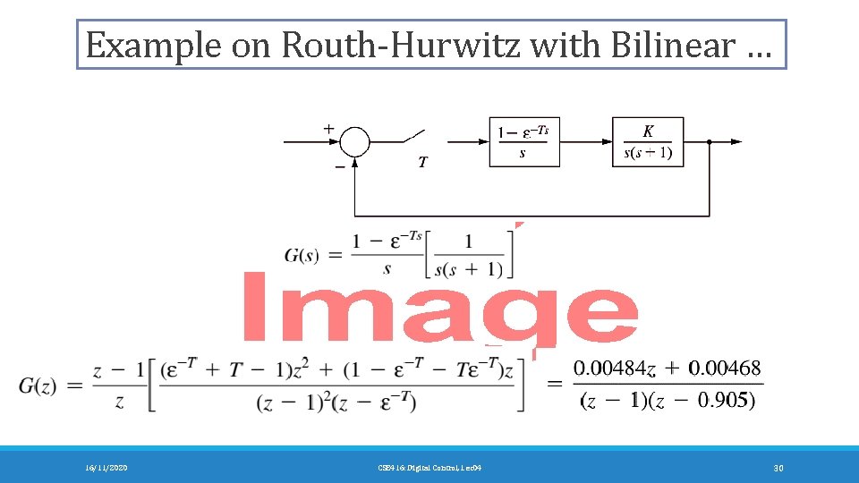
Example on Routh-Hurwitz with Bilinear … 16/11/2020 CSE 416: Digital Control, Lec 04 30

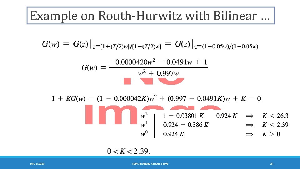
Example on Routh-Hurwitz with Bilinear … 16/11/2020 CSE 416: Digital Control, Lec 04 31

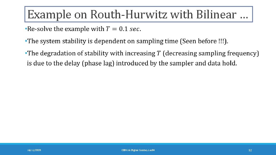
Example on Routh-Hurwitz with Bilinear … 16/11/2020 CSE 416: Digital Control, Lec 04 32

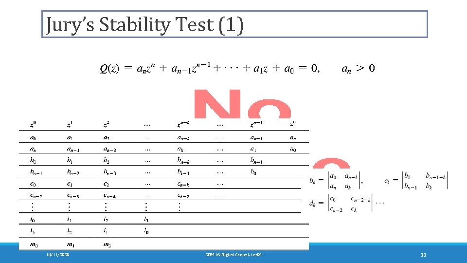
Jury’s Stability Test (1) 16/11/2020 CSE 416: Digital Control, Lec 04 33

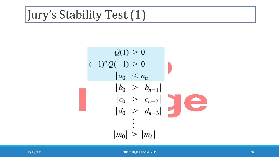
Jury’s Stability Test (1) 16/11/2020 CSE 416: Digital Control, Lec 04 34

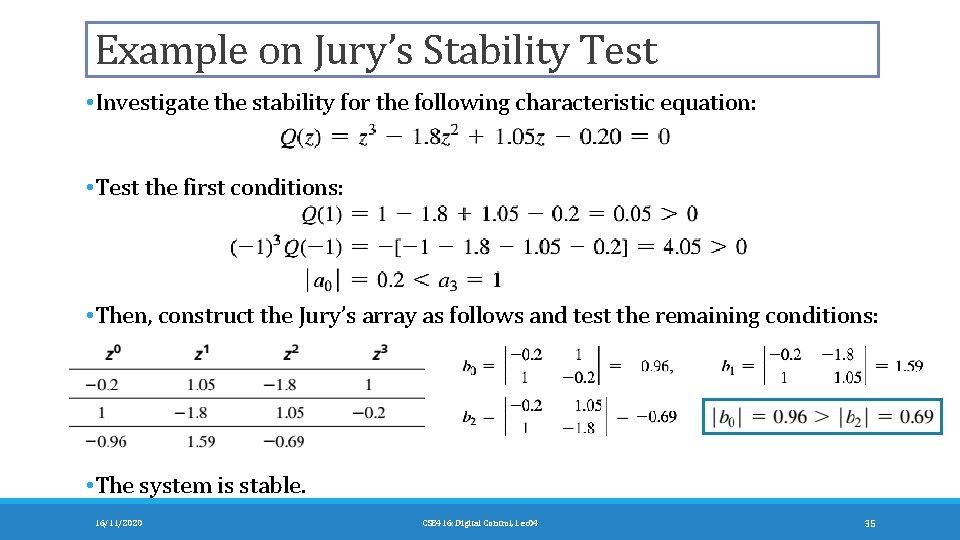
Example on Jury’s Stability Test • Investigate the stability for the following characteristic equation: • Test the first conditions: • Then, construct the Jury’s array as follows and test the remaining conditions: • The system is stable. 16/11/2020 CSE 416: Digital Control, Lec 04 35

Reading • Read Chapter 6. • Read Sections 7. 1 to 7. 5. 16/11/2020 CSE 416: Digital Control, Lec 04 36