CS 267 Sources of Parallelism and Locality in

CS 267 Sources of Parallelism and Locality in Simulation – Part 2 James Demmel www. cs. berkeley. edu/~demmel/cs 267_Spr 05 02/09/2005 CS 267 Lecture 7 1

Recap of Last Lecture • 4 kinds of simulations • • Discrete Event Systems Particle Systems Ordinary Differential Equations (ODEs) Today: Partial Differential Equations (PDEs) • Common problems: • Load balancing • • Dynamically, if load changes significantly during run Statically – Graph Partitioning – Sparse Matrix Vector Multiply (Sp. MV) • Linear Algebra • • Solving linear systems of equations, eigenvalue problems Sparse and dense matrices • Fast Particle Methods • 02/09/05 Solving in O(n) instead of O(n 2) CS 267 Lecture 7 2

Partial Differential Equations PDEs 02/09/2005 CS 267 Lecture 7 3

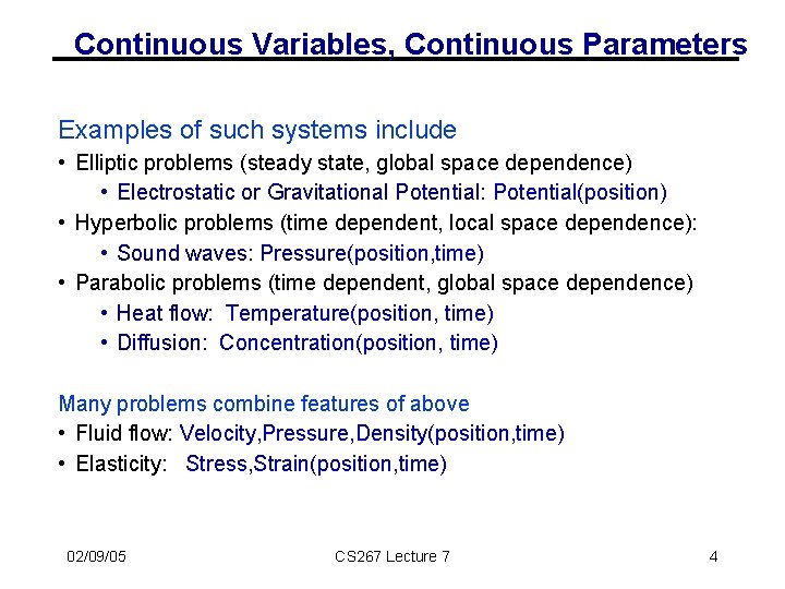
Continuous Variables, Continuous Parameters Examples of such systems include • Elliptic problems (steady state, global space dependence) • Electrostatic or Gravitational Potential: Potential(position) • Hyperbolic problems (time dependent, local space dependence): • Sound waves: Pressure(position, time) • Parabolic problems (time dependent, global space dependence) • Heat flow: Temperature(position, time) • Diffusion: Concentration(position, time) Many problems combine features of above • Fluid flow: Velocity, Pressure, Density(position, time) • Elasticity: Stress, Strain(position, time) 02/09/05 CS 267 Lecture 7 4

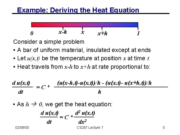
Example: Deriving the Heat Equation x-h x 0 x+h 1 Consider a simple problem • A bar of uniform material, insulated except at ends • Let u(x, t) be the temperature at position x at time t • Heat travels from x-h to x+h at rate proportional to: d u(x, t) dt =C* (u(x-h, t)-u(x, t))/h - (u(x, t)- u(x+h, t))/h h • As h 0, we get the heat equation: d u(x, t) d 2 u(x, t) =C* dt dx 2 02/09/05 CS 267 Lecture 7 5

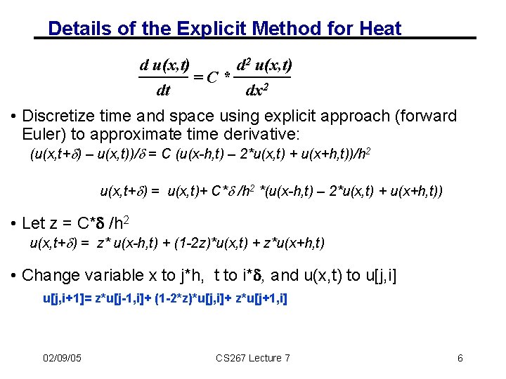
Details of the Explicit Method for Heat d u(x, t) dt =C* d 2 u(x, t) dx 2 • Discretize time and space using explicit approach (forward Euler) to approximate time derivative: (u(x, t+ ) – u(x, t))/ = C (u(x-h, t) – 2*u(x, t) + u(x+h, t))/h 2 u(x, t+ ) = u(x, t)+ C* /h 2 *(u(x-h, t) – 2*u(x, t) + u(x+h, t)) • Let z = C* /h 2 u(x, t+ ) = z* u(x-h, t) + (1 -2 z)*u(x, t) + z*u(x+h, t) • Change variable x to j*h, t to i* , and u(x, t) to u[j, i] u[j, i+1]= z*u[j-1, i]+ (1 -2*z)*u[j, i]+ z*u[j+1, i] 02/09/05 CS 267 Lecture 7 6

Explicit Solution of the Heat Equation • Use finite differences with u[j, i] as the temperature at • time t= i* (i = 0, 1, 2, …) and position x = j*h (j=0, 1, …, N=1/h) • initial conditions on u[j, 0] • boundary conditions on u[0, i] and u[N, i] i • At each timestep i = 0, 1, 2, . . . For j=0 to N i=5 u[j, i+1]= z*u[j-1, i]+ (1 -2*z)*u[j, i] + z*u[j+1, i] where z =C* /h 2 i=4 i=3 • This corresponds to i=2 • matrix vector multiply by T (next slide) • Combine nearest neighbors on grid i=1 j i=0 u[0, 0] u[1, 0] u[2, 0] u[3, 0] u[4, 0] u[5, 0] 02/09/05 CS 267 Lecture 7 7

Matrix View of Explicit Method for Heat • u[j, i+1]= z*u[j-1, i]+ (1 -2*z)*u[j, i] + z*u[j+1, i] • u[ : , i+1] = T * u[ : , i] where T is tridiagonal: 1 -2 z z T= z 1 -2 z z z = I – z*L, L= 2 -1 -1 2 1 -2 z Graph and “ 3 point stencil” z 1 -2 z z • L called Laplacian (in 1 D) • For a 2 D mesh (5 point stencil) the Laplacian is pentadiagonal • More on the matrix/grid views later 02/09/05 CS 267 Lecture 7 8

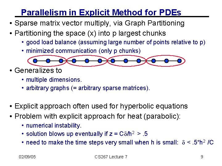
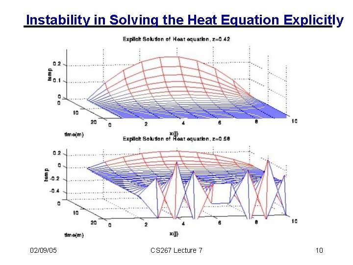
Parallelism in Explicit Method for PDEs • Sparse matrix vector multiply, via Graph Partitioning • Partitioning the space (x) into p largest chunks • good load balance (assuming large number of points relative to p) • minimized communication (only p chunks) • Generalizes to • multiple dimensions. • arbitrary graphs (= arbitrary sparse matrices). • Explicit approach often used for hyperbolic equations • Problem with explicit approach for heat (parabolic): • numerical instability. • solution blows up eventually if z = C /h 2 >. 5 • need to make the time steps very small when h is small: <. 5*h 2 /C 02/09/05 CS 267 Lecture 7 9

Instability in Solving the Heat Equation Explicitly 02/09/05 CS 267 Lecture 7 10

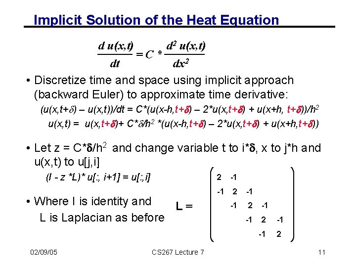
Implicit Solution of the Heat Equation d u(x, t) =C* d 2 u(x, t) dt dx 2 • Discretize time and space using implicit approach (backward Euler) to approximate time derivative: (u(x, t+ ) – u(x, t))/dt = C*(u(x-h, t+ ) – 2*u(x, t+ ) + u(x+h, t+ ))/h 2 u(x, t) = u(x, t+ )+ C* /h 2 *(u(x-h, t+ ) – 2*u(x, t+ ) + u(x+h, t+ )) • Let z = C* /h 2 and change variable t to i* , x to j*h and u(x, t) to u[j, i] (I - z *L)* u[: , i+1] = u[: , i] • Where I is identity and L= L is Laplacian as before 02/09/05 CS 267 Lecture 7 2 -1 -1 2 11

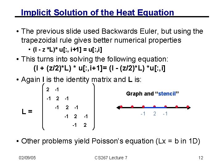
Implicit Solution of the Heat Equation • The previous slide used Backwards Euler, but using the trapezoidal rule gives better numerical properties • (I - z *L)* u[: , i+1] = u[: , i] • This turns into solving the following equation: (I + (z/2)*L) * u[: , i+1]= (I - (z/2)*L) *u[: , i] • Again I is the identity matrix and L is: L= 2 -1 -1 2 Graph and “stencil” -1 2 -1 • Other problems yield Poisson’s equation (Lx = b in 1 D) 02/09/05 CS 267 Lecture 7 12

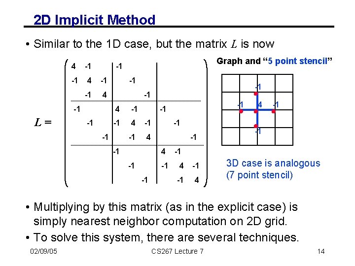
2 D Implicit Method • Similar to the 1 D case, but the matrix L is now 4 -1 -1 4 -1 L= Graph and “ 5 point stencil” -1 -1 -1 4 -1 -1 -1 4 -1 -1 4 3 D case is analogous (7 point stencil) • Multiplying by this matrix (as in the explicit case) is simply nearest neighbor computation on 2 D grid. • To solve this system, there are several techniques. 02/09/05 CS 267 Lecture 7 14

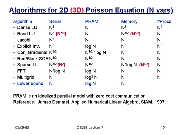
Algorithms for 2 D (3 D) Poisson Equation (N vars) Algorithm Serial • Dense LU N 3 • Band LU N 2 (N 7/3) • Jacobi N 2 2 • Explicit Inv. N • Conj. Gradients N 3/2 • Red/Black SOR N 3/2 • Sparse LU N 3/2 (N 2) • FFT N*log N • Multigrid N • Lower bound N PRAM N N N log N N 1/2 *log N N 1/2 log N log 2 N log N Memory N 2 N 3/2 (N 5/3) N 2 N N*log N (N 4/3) N N N #Procs N 2 N N N N PRAM is an idealized parallel model with zero cost communication Reference: James Demmel, Applied Numerical Linear Algebra, SIAM, 1997. 02/09/05 CS 267 Lecture 7 15

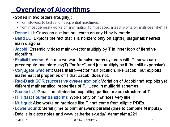
Overview of Algorithms • Sorted in two orders (roughly): • from slowest to fastest on sequential machines. • from most general (works on any matrix) to most specialized (works on matrices “like” T). • Dense LU: Gaussian elimination; works on any N-by-N matrix. • Band LU: Exploits the fact that T is nonzero only on sqrt(N) diagonals nearest main diagonal. • Jacobi: Essentially does matrix-vector multiply by T in inner loop of iterative algorithm. • Explicit Inverse: Assume we want to solve many systems with T, so we can precompute and store inv(T) “for free”, and just multiply by it (but still expensive). • Conjugate Gradient: Uses matrix-vector multiplication, like Jacobi, but exploits mathematical properties of T that Jacobi does not. • Red-Black SOR (successive over-relaxation): Variation of Jacobi that exploits yet different mathematical properties of T. Used in multigrid schemes. • Sparse LU: Gaussian elimination exploiting particular zero structure of T. • FFT (fast Fourier transform): Works only on matrices very like T. • Multigrid: Also works on matrices like T, that come from elliptic PDEs. • Lower Bound: Serial (time to print answer); parallel (time to combine N inputs). • Details in class notes and www. cs. berkeley. edu/~demmel/ma 221. 02/09/05 CS 267 Lecture 7 16

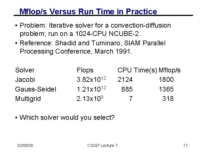
Mflop/s Versus Run Time in Practice • Problem: Iterative solver for a convection-diffusion problem; run on a 1024 -CPU NCUBE-2. • Reference: Shadid and Tuminaro, SIAM Parallel Processing Conference, March 1991. Solver Jacobi Gauss-Seidel Multigrid Flops 3. 82 x 1012 1. 21 x 1012 2. 13 x 109 CPU Time(s) Mflop/s 2124 1800 885 1365 7 318 • Which solver would you select? 02/09/05 CS 267 Lecture 7 17

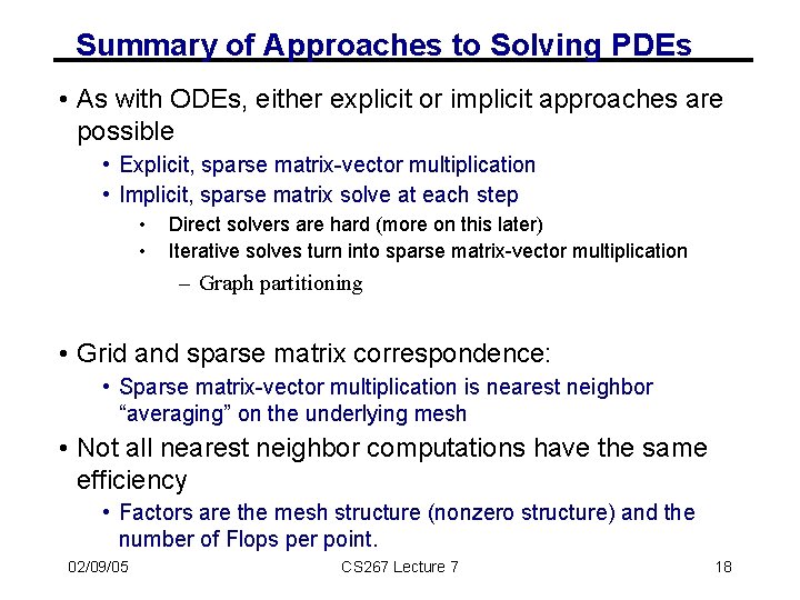
Summary of Approaches to Solving PDEs • As with ODEs, either explicit or implicit approaches are possible • Explicit, sparse matrix-vector multiplication • Implicit, sparse matrix solve at each step • • Direct solvers are hard (more on this later) Iterative solves turn into sparse matrix-vector multiplication – Graph partitioning • Grid and sparse matrix correspondence: • Sparse matrix-vector multiplication is nearest neighbor “averaging” on the underlying mesh • Not all nearest neighbor computations have the same efficiency • Factors are the mesh structure (nonzero structure) and the number of Flops per point. 02/09/05 CS 267 Lecture 7 18

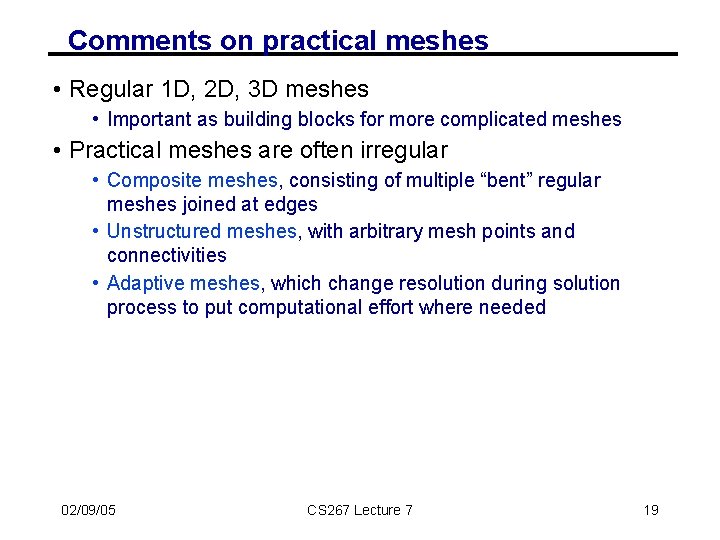
Comments on practical meshes • Regular 1 D, 2 D, 3 D meshes • Important as building blocks for more complicated meshes • Practical meshes are often irregular • Composite meshes, consisting of multiple “bent” regular meshes joined at edges • Unstructured meshes, with arbitrary mesh points and connectivities • Adaptive meshes, which change resolution during solution process to put computational effort where needed 02/09/05 CS 267 Lecture 7 19

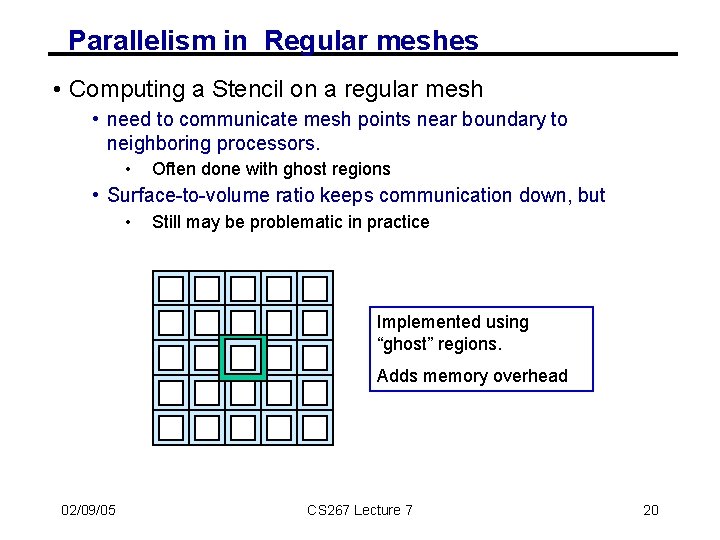
Parallelism in Regular meshes • Computing a Stencil on a regular mesh • need to communicate mesh points near boundary to neighboring processors. • Often done with ghost regions • Surface-to-volume ratio keeps communication down, but • Still may be problematic in practice Implemented using “ghost” regions. Adds memory overhead 02/09/05 CS 267 Lecture 7 20

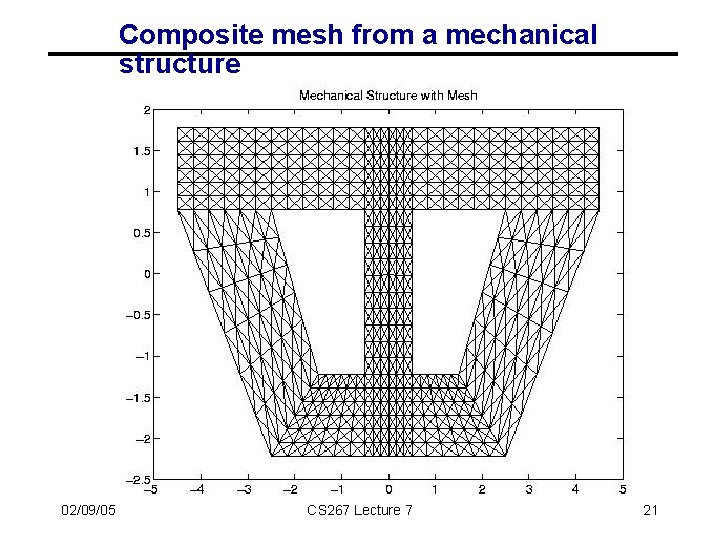
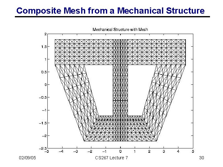
Composite mesh from a mechanical structure 02/09/05 CS 267 Lecture 7 21

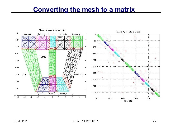
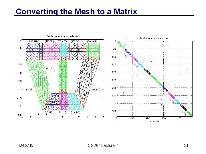
Converting the mesh to a matrix 02/09/05 CS 267 Lecture 7 22

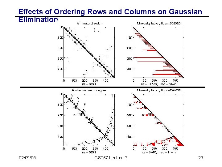
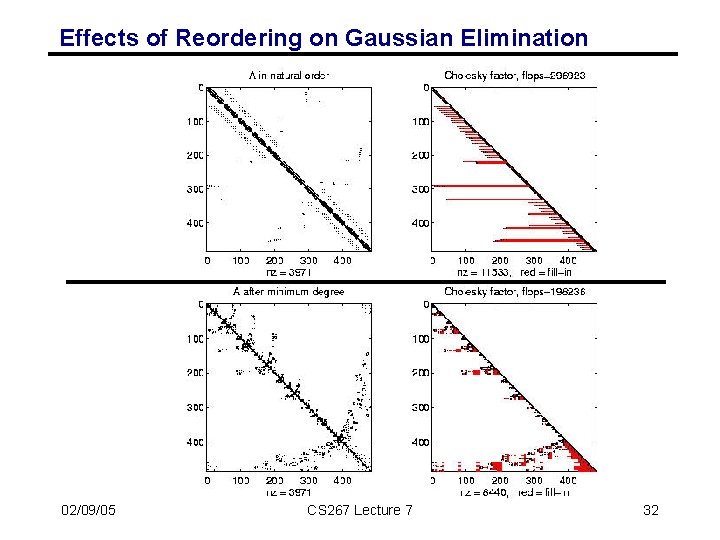
Effects of Ordering Rows and Columns on Gaussian Elimination 02/09/05 CS 267 Lecture 7 23

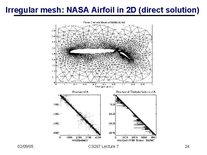
Irregular mesh: NASA Airfoil in 2 D (direct solution) 02/09/05 CS 267 Lecture 7 24

Irregular mesh: Tapered Tube (multigrid) 02/09/05 CS 267 Lecture 7 25

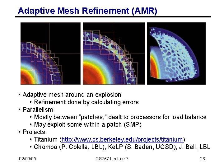
Adaptive Mesh Refinement (AMR) • Adaptive mesh around an explosion • Refinement done by calculating errors • Parallelism • Mostly between “patches, ” dealt to processors for load balance • May exploit some within a patch (SMP) • Projects: • Titanium (http: //www. cs. berkeley. edu/projects/titanium) • Chombo (P. Colella, LBL), Ke. LP (S. Baden, UCSD), J. Bell, LBL 02/09/05 CS 267 Lecture 7 26

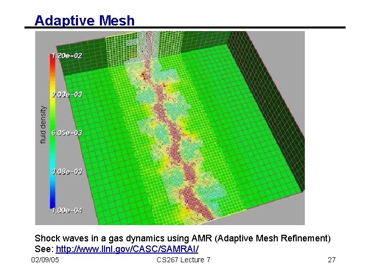
fluid density Adaptive Mesh Shock waves in a gas dynamics using AMR (Adaptive Mesh Refinement) See: http: //www. llnl. gov/CASC/SAMRAI/ 02/09/05 CS 267 Lecture 7 27

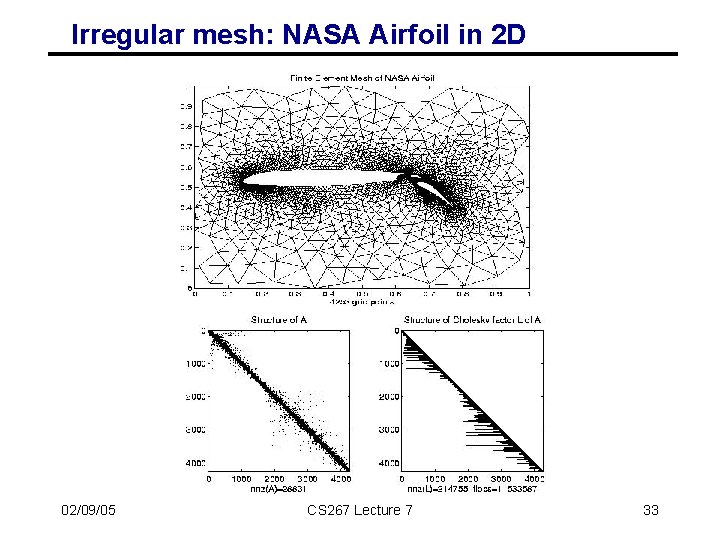
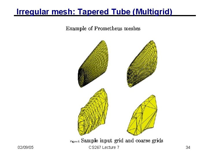
Challenges of Irregular Meshes • How to generate them in the first place • Triangle, a 2 D mesh partitioner by Jonathan Shewchuk • 3 D harder! • How to partition them • Par. Metis, a parallel graph partitioner • How to design iterative solvers • PETSc, a Portable Extensible Toolkit for Scientific Computing • Prometheus, a multigrid solver for finite element problems on irregular meshes • How to design direct solvers • Super. LU, parallel sparse Gaussian elimination • These are challenges to do sequentially, more so in parallel 02/09/05 CS 267 Lecture 7 28

Extra Slides 02/09/2005 CS 267 Lecture 7 29

Composite Mesh from a Mechanical Structure 02/09/05 CS 267 Lecture 7 30

Converting the Mesh to a Matrix 02/09/05 CS 267 Lecture 7 31

Effects of Reordering on Gaussian Elimination 02/09/05 CS 267 Lecture 7 32

Irregular mesh: NASA Airfoil in 2 D 02/09/05 CS 267 Lecture 7 33

Irregular mesh: Tapered Tube (Multigrid) 02/09/05 CS 267 Lecture 7 34

CS 267 Final Projects • Project proposal • • Teams of 3 students, typically across departments Interesting parallel application or system Conference-quality paper High performance is key: • Understanding performance, tuning, scaling, etc. • More important the difficulty of problem • Leverage • Projects in other classes (but discuss with me first) • Research projects 02/09/05 CS 267 Lecture 7 35

Project Ideas • Applications • Implement existing sequential or shared memory program on distributed memory • Investigate SMP trade-offs (using only MPI versus MPI and thread based parallelism) • Tools and Systems • Effects of reordering on sparse matrix factoring and solves • Numerical algorithms • Improved solver for immersed boundary method • Use of multiple vectors (blocked algorithms) in iterative solvers 02/09/05 CS 267 Lecture 7 36

Project Ideas • Novel computational platforms • • Exploiting hierarchy of SMP-clusters in benchmarks Computing aggregate operations on ad hoc networks (Culler) Push/explore limits of computing on “the grid” Performance under failures • Detailed benchmarking and performance analysis, including identification of optimization opportunities • Titanium • UPC • IBM SP (Blue Horizon) 02/09/05 CS 267 Lecture 7 37