Crystallography Lecture 22 Refinement and Validation Refinement Initial

Crystallography -- Lecture 22 Refinement and Validation

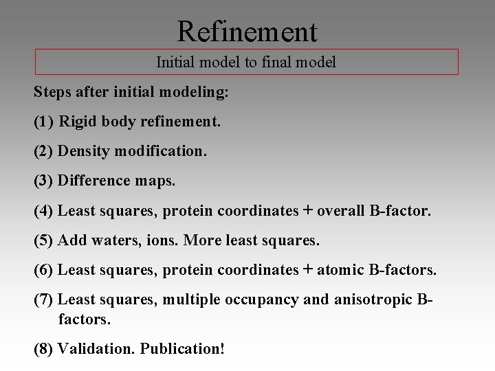
Refinement Initial model to final model Steps after initial modeling: (1) Rigid body refinement. (2) Density modification. (3) Difference maps. (4) Least squares, protein coordinates + overall B-factor. (5) Add waters, ions. More least squares. (6) Least squares, protein coordinates + atomic B-factors. (7) Least squares, multiple occupancy and anisotropic Bfactors. (8) Validation. Publication!

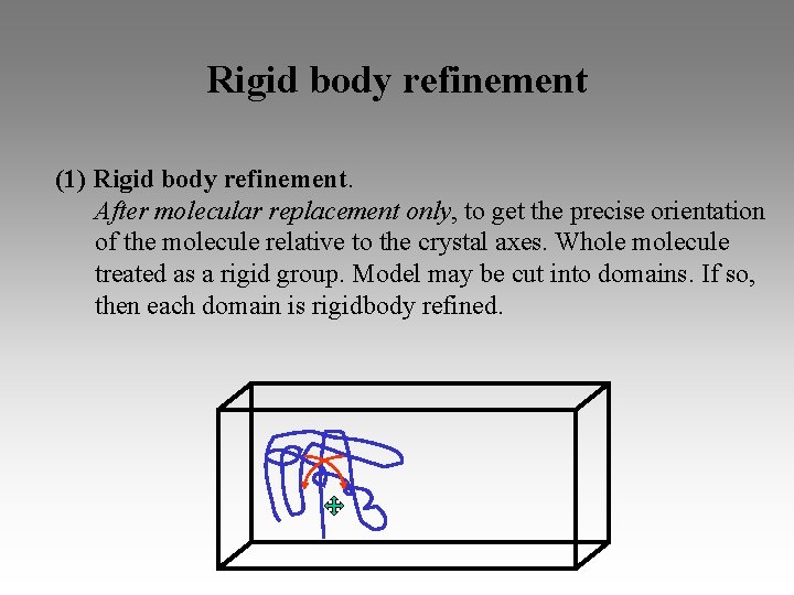
Rigid body refinement (1) Rigid body refinement. After molecular replacement only, to get the precise orientation of the molecule relative to the crystal axes. Whole molecule treated as a rigid group. Model may be cut into domains. If so, then each domain is rigidbody refined.

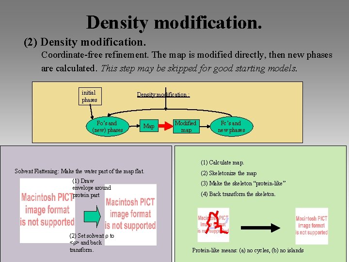
Density modification. (2) Density modification. Coordinate-free refinement. The map is modified directly, then new phases are calculated. This step may be skipped for good starting models. initial phases Fo’s and (new) phases Density modification : Map Modified map Fc’s and new phases (1) Calculate map. Solvent Flattening: Make the water part of the map flat. (1) Draw envelope around protein part (2) Set solvent to < > and back transform. (2) Skeletonize the map (3) Make the skeleton “protein-like” (4) Back transform the skeleton. Protein-like means: (a) no cycles, (b) no islands

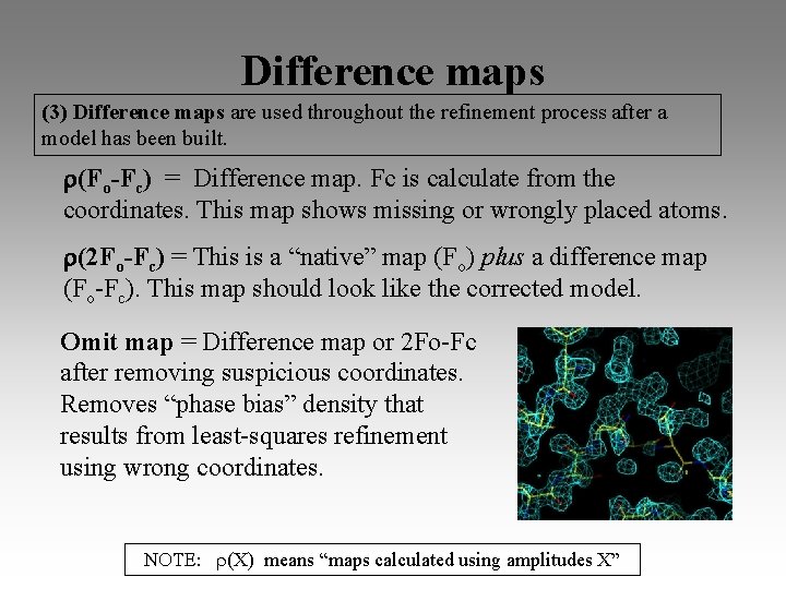
Difference maps (3) Difference maps are used throughout the refinement process after a model has been built. (Fo-Fc) = Difference map. Fc is calculate from the coordinates. This map shows missing or wrongly placed atoms. (2 Fo-Fc) = This is a “native” map (Fo) plus a difference map (Fo-Fc). This map should look like the corrected model. Omit map = Difference map or 2 Fo-Fc after removing suspicious coordinates. Removes “phase bias” density that results from least-squares refinement using wrong coordinates. (X) means “maps calculated using amplitudes X”

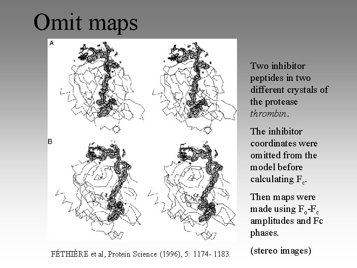
Omit maps Two inhibitor peptides in two different crystals of the protease thrombin. The inhibitor coordinates were omitted from the model before calculating Fc. Then maps were made using Fo-Fc amplitudes and Fc phases. FÉTHIÈRE et al, Protein Science (1996), 5: 1174 - 1183. (stereo images)

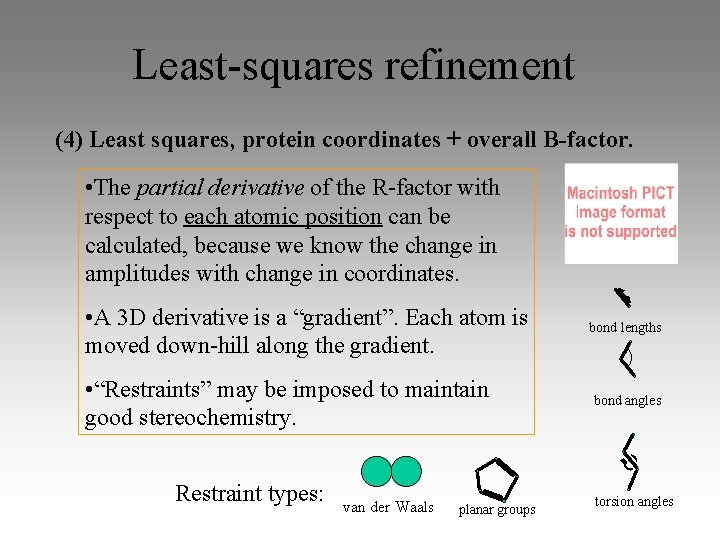
Least-squares refinement (4) Least squares, protein coordinates + overall B-factor. • The partial derivative of the R-factor with respect to each atomic position can be calculated, because we know the change in amplitudes with change in coordinates. • A 3 D derivative is a “gradient”. Each atom is moved down-hill along the gradient. • “Restraints” may be imposed to maintain good stereochemistry. Restraint types: van der Waals planar groups bond lengths bond angles torsion angles

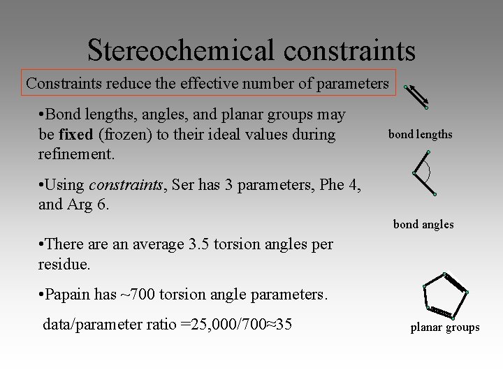
Stereochemical constraints Constraints reduce the effective number of parameters • Bond lengths, angles, and planar groups may be fixed (frozen) to their ideal values during refinement. bond lengths • Using constraints, Ser has 3 parameters, Phe 4, and Arg 6. bond angles • There an average 3. 5 torsion angles per residue. • Papain has ~700 torsion angle parameters. data/parameter ratio =25, 000/700≈35 planar groups

Adding waters, ions. (5) Add waters, ions. More least squares. Calculate difference map Place waters (just an oxygen) in the peak positive density position if (1) there is no atom there, (2) there is an atom nearby, (3) the density or shape does not suggest an ion of ligand.

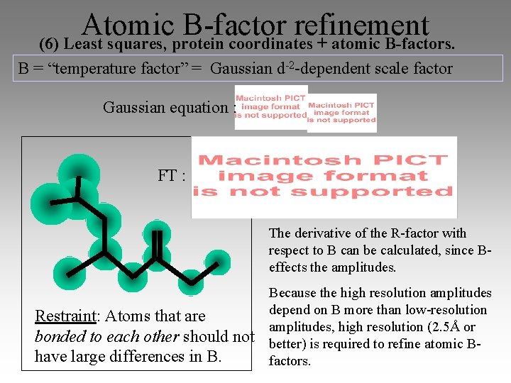
Atomic B-factor refinement (6) Least squares, protein coordinates + atomic B-factors. B = “temperature factor” = Gaussian d-2 -dependent scale factor Gaussian equation : FT : The derivative of the R-factor with respect to B can be calculated, since Beffects the amplitudes. Restraint: Atoms that are bonded to each other should not have large differences in B. Because the high resolution amplitudes depend on B more than low-resolution amplitudes, high resolution (2. 5Å or better) is required to refine atomic Bfactors.

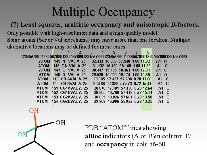
Multiple Occupancy (7) Least squares, multiple occupancy and anisotropic B-factors. Only possible with high-resolution data and a high-quality model. Some atoms (Ser or Val sidechains) may have more than one location. Multiple alternative locations may be defined for these cases. 1 2 3 4 5 6 7 8 1234567890123456789012345678901234567890 ATOM 145 N VAL A 25 32. 433 16. 336 57. 540 1. 00 11. 92 A 1 N ATOM 146 CA VAL A 25 31. 132 16. 439 58. 160 1. 00 11. 85 A 1 C ATOM 147 C VAL A 25 30. 447 15. 105 58. 363 1. 00 12. 34 A 1 C ATOM 148 O VAL A 25 29. 520 15. 059 59. 174 1. 00 15. 65 A 1 O ATOM 149 CB AVAL A 25 30. 385 17. 437 57. 230 0. 28 13. 88 A 1 C ATOM 150 CB BVAL A 25 30. 166 17. 399 57. 373 0. 72 15. 41 A 1 C ATOM 151 CG 1 AVAL A 25 28. 870 17. 401 57. 336 0. 28 12. 64 A 1 C ATOM 152 CG 1 BVAL A 25 30. 805 18. 788 57. 449 0. 72 15. 11 A 1 C ATOM 153 CG 2 AVAL A 25 30. 835 18. 826 57. 661 0. 28 13. 58 A 1 C ATOM 154 CG 2 BVAL A 25 29. 909 16. 996 55. 922 0. 72 13. 25 A 1 C OH OH OH PDB “ATOM” lines showing altloc indicators (A or B)in column 17 and occupancy in cols 56 -60.

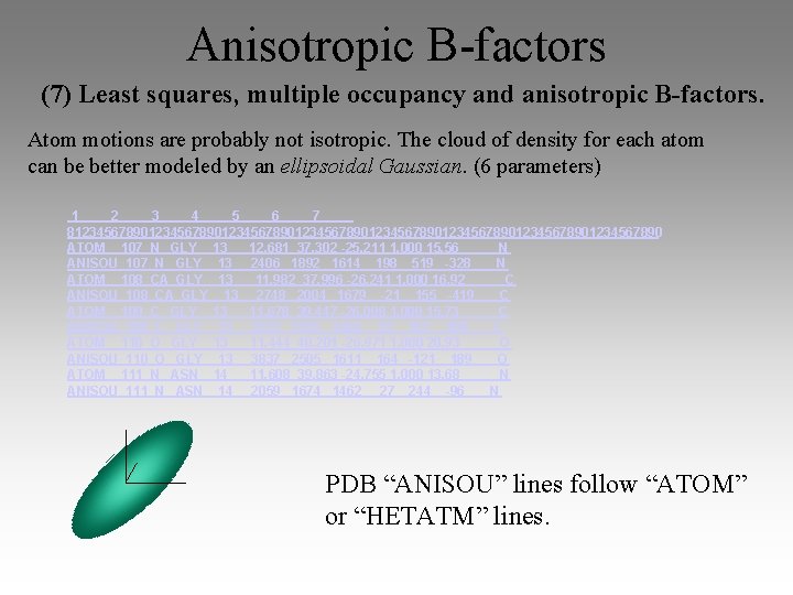
Anisotropic B-factors (7) Least squares, multiple occupancy and anisotropic B-factors. Atom motions are probably not isotropic. The cloud of density for each atom can be better modeled by an ellipsoidal Gaussian. (6 parameters) 1 2 3 4 5 6 7 81234567890123456789012345678901234567890 ATOM 107 N GLY 13 12. 681 37. 302 -25. 211 1. 000 15. 56 N ANISOU 107 N GLY 13 2406 1892 1614 198 519 -328 N ATOM 108 CA GLY 13 11. 982 37. 996 -26. 241 1. 000 16. 92 C ANISOU 108 CA GLY 13 2748 2004 1679 -21 155 -419 C ATOM 109 C GLY 13 11. 678 39. 447 -26. 008 1. 000 15. 73 C ANISOU 109 C GLY 13 2555 1955 1468 87 357 -109 C ATOM 110 O GLY 13 11. 444 40. 201 -26. 971 1. 000 20. 93 O ANISOU 110 O GLY 13 3837 2505 1611 164 -121 189 O ATOM 111 N ASN 14 11. 608 39. 863 -24. 755 1. 000 13. 68 N ANISOU 111 N ASN 14 2059 1674 1462 27 244 -96 N PDB “ANISOU” lines follow “ATOM” or “HETATM” lines.

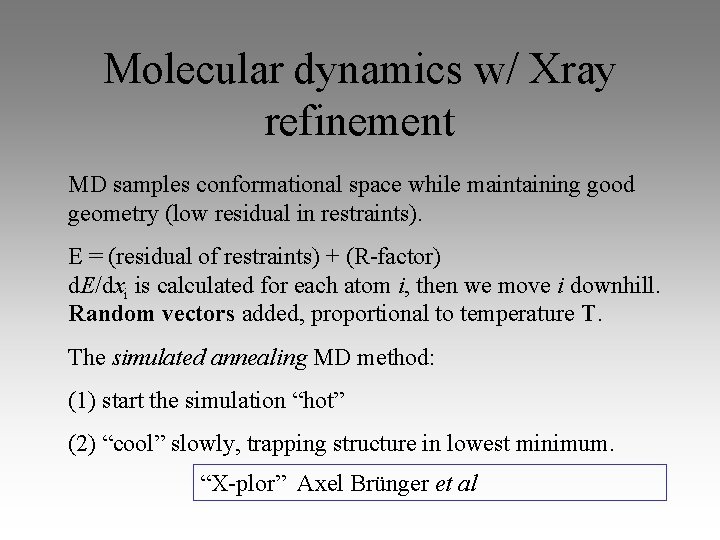
Molecular dynamics w/ Xray refinement MD samples conformational space while maintaining good geometry (low residual in restraints). E = (residual of restraints) + (R-factor) d. E/dxi is calculated for each atom i, then we move i downhill. Random vectors added, proportional to temperature T. The simulated annealing MD method: (1) start the simulation “hot” (2) “cool” slowly, trapping structure in lowest minimum. “X-plor” Axel Brünger et al

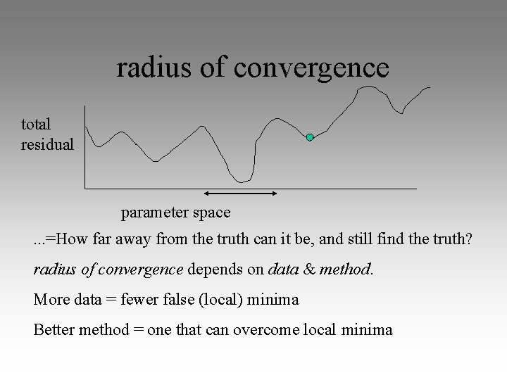
radius of convergence total residual parameter space. . . =How far away from the truth can it be, and still find the truth? radius of convergence depends on data & method. More data = fewer false (local) minima Better method = one that can overcome local minima

The final model www. rcsb. org

Errors and Validation

Sources of error • Error is broadly defined as the difference between your model and reality. • Sources of error can be in the data (the crystal itself or the processing of the data) or in the molecular model. • If the model is at fault, errors may be localized to certain parts of a model, or spread throughout.

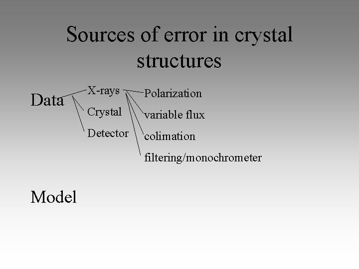
Sources of error in crystal structures Data X-rays Polarization Crystal variable flux Detector colimation filtering/monochrometer Model

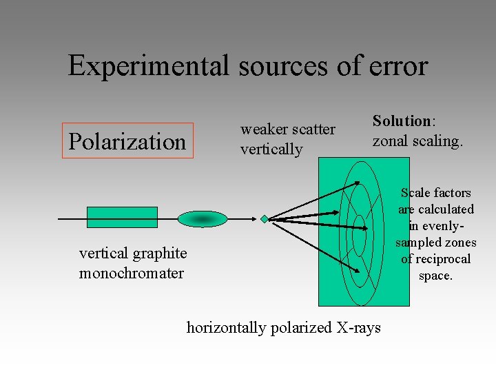
Experimental sources of error Polarization weaker scatter vertically Solution: zonal scaling. vertical graphite monochromater horizontally polarized X-rays Scale factors are calculated in evenlysampled zones of reciprocal space.

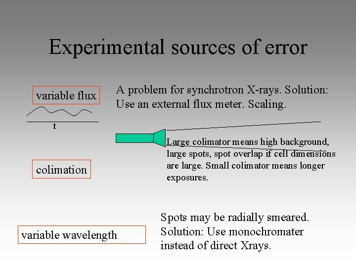
Experimental sources of error variable flux A problem for synchrotron X-rays. Solution: Use an external flux meter. Scaling. t colimation variable wavelength Large colimator means high background, large spots, spot overlap if cell dimensions are large. Small colimator means longer exposures. Spots may be radially smeared. Solution: Use monochromater instead of direct Xrays.

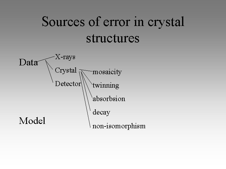
Sources of error in crystal structures Data X-rays Crystal mosaicity Detector twinning absorbsion Model decay non-isomorphism

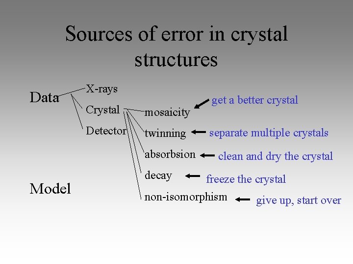
Sources of error in crystal structures Data X-rays Crystal mosaicity Detector twinning absorbsion Model decay get a better crystal separate multiple crystals clean and dry the crystal freeze the crystal non-isomorphism give up, start over

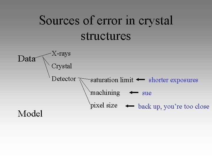
Sources of error in crystal structures Data X-rays Crystal Detector saturation limit machining Model pixel size shorter exposures sue back up, you’re too close

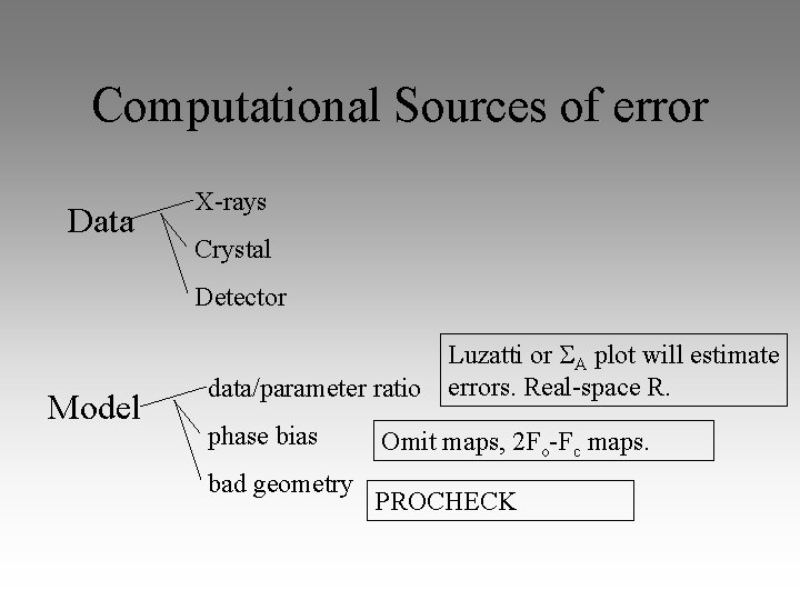
Computational Sources of error Data X-rays Crystal Detector Model Luzatti or A plot will estimate data/parameter ratio errors. Real-space R. phase bias bad geometry Omit maps, 2 Fo-Fc maps. PROCHECK

Cross-validation: The free R-factor The R-factor measures the residual difference between observed and calculated amplitudes. Free R is summed on a “test set”. Test set data was not used for refinement. Free R ask: “How well does your model predict the data it hasn’t been fit to? ” Note: T = independent test set of F’s.

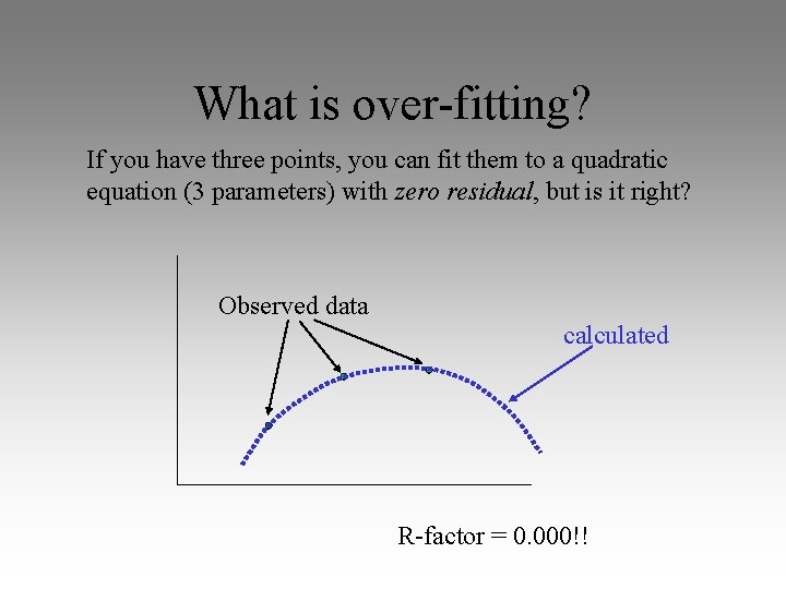
What is over-fitting? If you have three points, you can fit them to a quadratic equation (3 parameters) with zero residual, but is it right? Observed data calculated R-factor = 0. 000!!

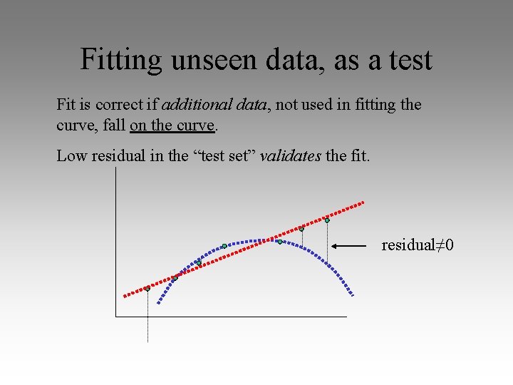
Fitting unseen data, as a test Fit is correct if additional data, not used in fitting the curve, fall on the curve. Low residual in the “test set” validates the fit. residual≠ 0

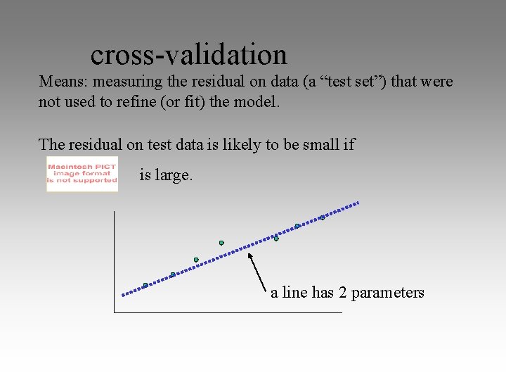
cross-validation Means: measuring the residual on data (a “test set”) that were not used to refine (or fit) the model. The residual on test data is likely to be small if is large. a line has 2 parameters

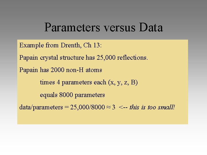
Parameters versus Data Example from Drenth, Ch 13: Papain crystal structure has 25, 000 reflections. Papain has 2000 non-H atoms times 4 parameters each (x, y, z, B) equals 8000 parameters data/parameters = 25, 000/8000 ≈ 3 <-- this is too small!

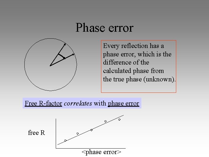
Phase error Every reflection has a phase error, which is the difference of the calculated phase from the true phase (unknown). Free R-factor correlates with phase error free R <phase error>

Thought experiment What is the phase error for 4Å resolution reflections if the average coordinate error is 1Å?

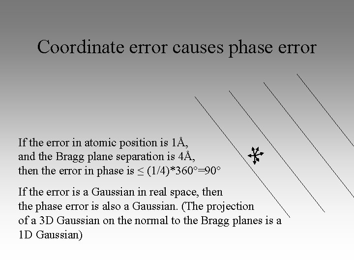
Coordinate error causes phase error If the error in atomic position is 1Å, and the Bragg plane separation is 4Å, then the error in phase is ≤ (1/4)*360°=90° If the error is a Gaussian in real space, then the phase error is also a Gaussian. (The projection of a 3 D Gaussian on the normal to the Bragg planes is a 1 D Gaussian)

Luzzati plot Data is divided into shells in S (=1/d). The R-factor for each shell is calculated and plotted. The plot is matched to theoretical R vs S for a model with randomlydistributed errors = e. ps. Luzzati did this in 1952, long before computers!

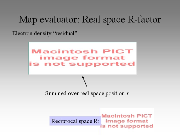
Map evaluator: Real space R-factor Electron density “residual” Summed over real space position r Reciprocal space R:

Real space R-factor as a diagnostic High B-factors or real-space R may indicate places where the model is locally wrong.

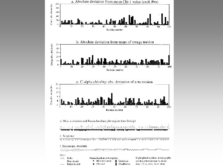
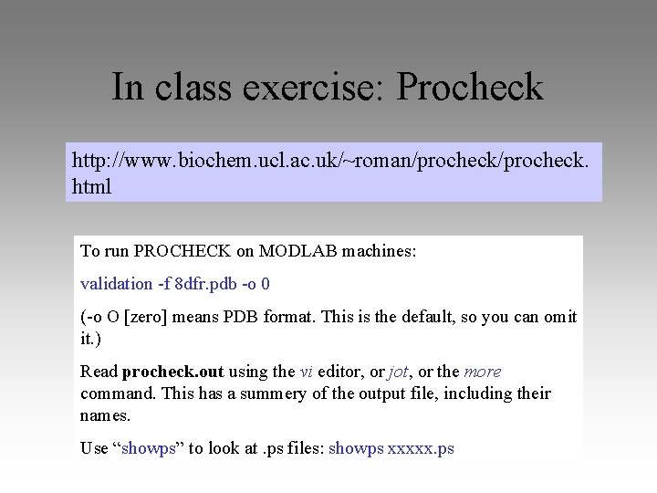
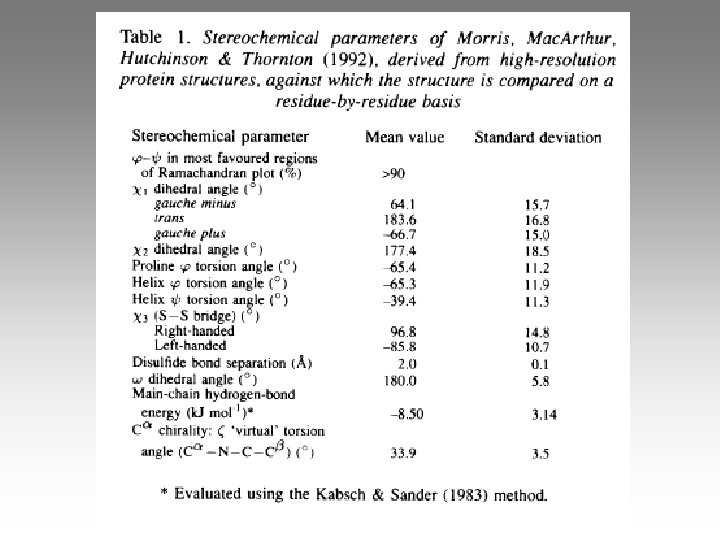
In class exercise: Procheck http: //www. biochem. ucl. ac. uk/~roman/procheck. html To run PROCHECK on MODLAB machines: validation -f 8 dfr. pdb -o 0 (-o O [zero] means PDB format. This is the default, so you can omit it. ) Read procheck. out using the vi editor, or jot, or the more command. This has a summery of the output file, including their names. Use “showps” to look at. ps files: showps xxxxx. ps

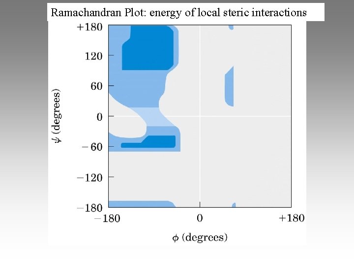
Ramachandran Plot: energy of local steric interactions

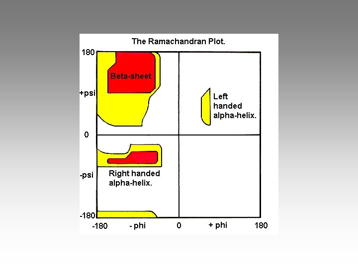
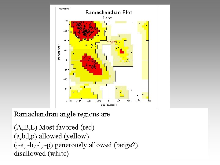
Ramachandran angle regions are (A, B, L) Most favored (red) (a, b, l, p) allowed (yellow) (~a, ~b, ~l, ~p) generously allowed (beige? ) disallowed (white)

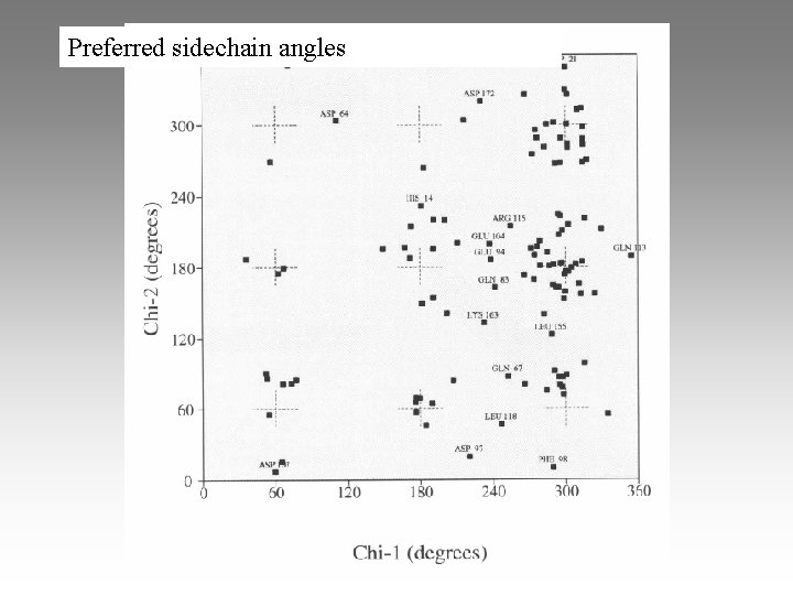
Preferred sidechain angles