Crosstalk Calculation and SLEM 2 Topics Crosstalk and

Crosstalk Calculation and SLEM

2 Topics § Crosstalk and Impedance § Superposition § Examples § SLEM Crosstalk Calculation

Cross Talk and Impedance is an electromagnetic parameter and is therefore effected by the electromagnetic environment as shown in the preceding slides. In the this second half, we will focus on looking at cross talk as a function of impedance and some of the benefits of viewing cross talk from this perspective. Crosstalk Calculation 3

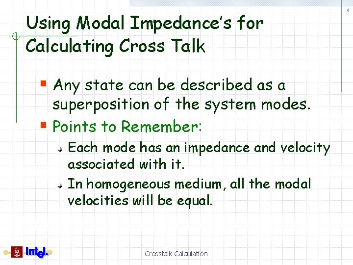
Using Modal Impedance’s for Calculating Cross Talk § Any state can be described as a superposition of the system modes. § Points to Remember: Each mode has an impedance and velocity associated with it. In homogeneous medium, all the modal velocities will be equal. Crosstalk Calculation 4

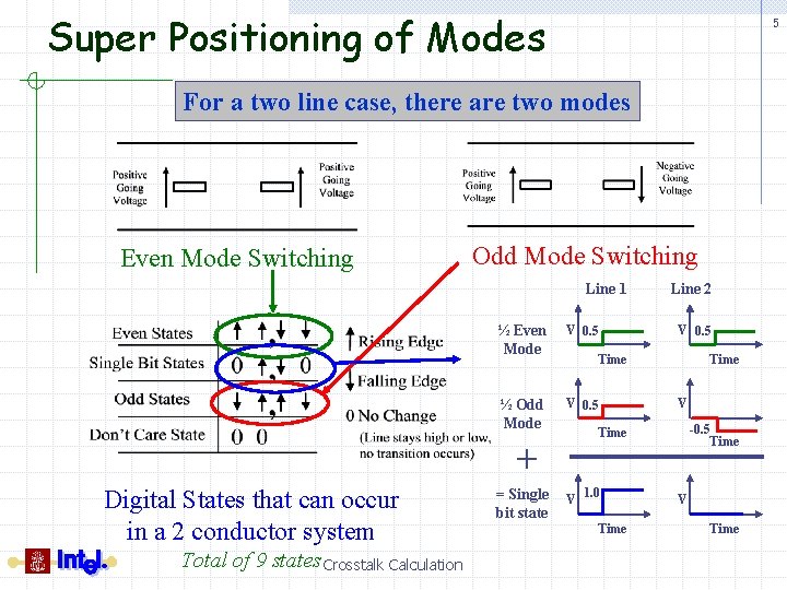
Super Positioning of Modes 5 For a two line case, there are two modes Even Mode Switching Odd Mode Switching Line 1 ½ Even Mode V 0. 5 ½ Odd Mode V 0. 5 Total of 9 states Crosstalk Calculation = Single bit state V 0. 5 Time V -0. 5 Time + Digital States that can occur in a 2 conductor system Line 2 V 1. 0 Time V Time

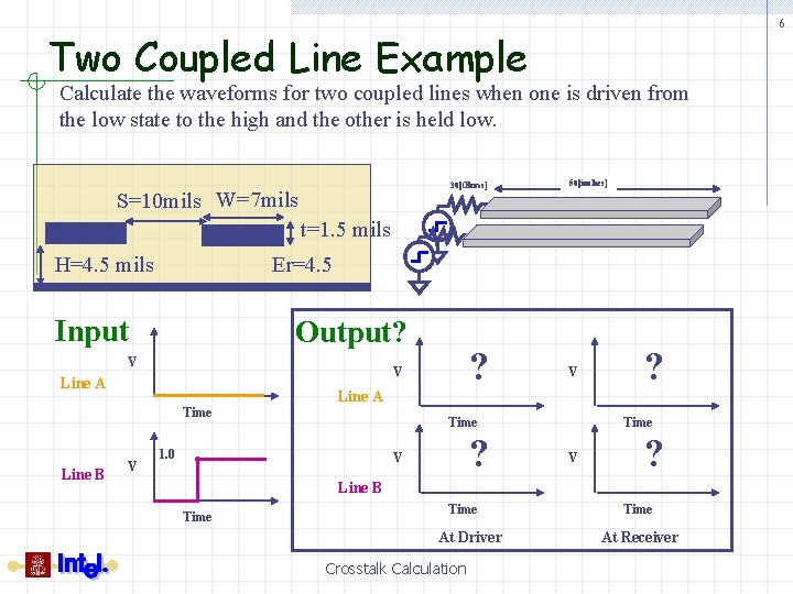
6 Two Coupled Line Example Calculate the waveforms for two coupled lines when one is driven from the low state to the high and the other is held low. 30[Ohms] S=10 mils W=7 mils 50[inches] t=1. 5 mils H=4. 5 mils Er=4. 5 Input Output? V Line A Time Line B ? V Line A V V Time 1. 0 ? V ? Time V ? Line B Time At Driver Crosstalk Calculation Time At Receiver

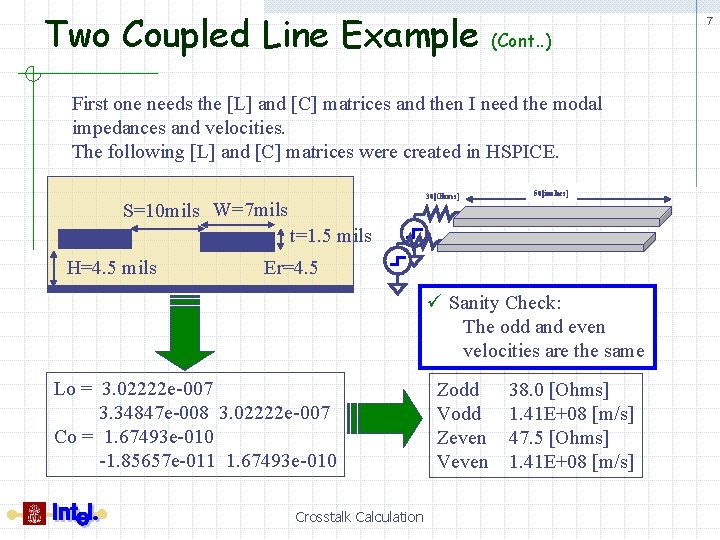
Two Coupled Line Example (Cont. . ) First one needs the [L] and [C] matrices and then I need the modal impedances and velocities. The following [L] and [C] matrices were created in HSPICE. 30[Ohms] S=10 mils W=7 mils 50[inches] t=1. 5 mils H=4. 5 mils Er=4. 5 ü Sanity Check: The odd and even velocities are the same Lo = 3. 02222 e-007 3. 34847 e-008 3. 02222 e-007 Co = 1. 67493 e-010 -1. 85657 e-011 1. 67493 e-010 Crosstalk Calculation Zodd Vodd Zeven Veven 38. 0 [Ohms] 1. 41 E+08 [m/s] 47. 5 [Ohms] 1. 41 E+08 [m/s] 7

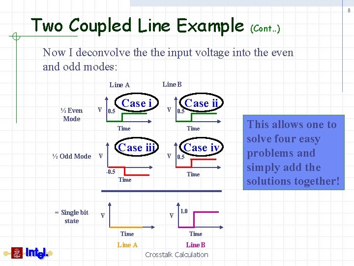
Two Coupled Line Example 8 (Cont. . ) Now I deconvolve the input voltage into the even and odd modes: Line B Line A ½ Even Mode V 0. 5 Case i V Case ii 0. 5 Time ½ Odd Mode Time Case iii V V -0. 5 V V Time Line A 0. 5 Time = Single bit state Case iv 1. 0 Time Line B Crosstalk Calculation This allows one to solve four easy problems and simply add the solutions together!

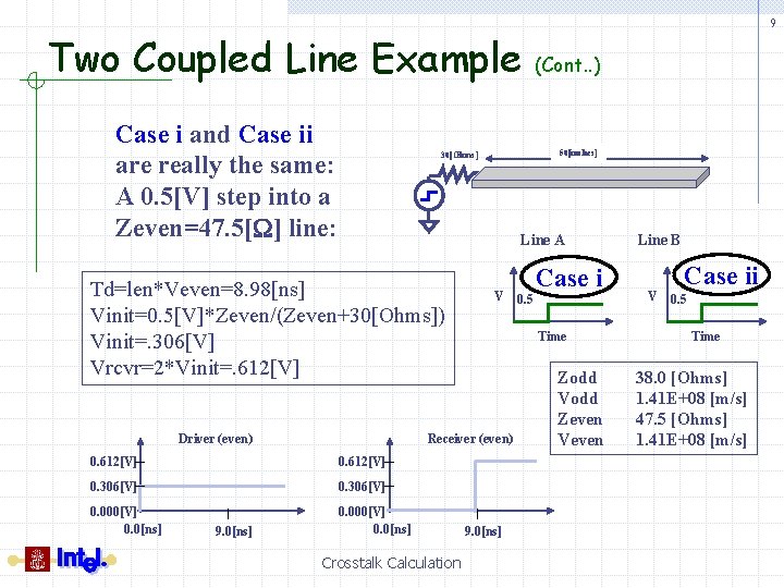
Two Coupled Line Example Case i and Case ii are really the same: A 0. 5[V] step into a Zeven=47. 5[W] line: (Cont. . ) 50[inches] 30[Ohms] Line A Td=len*Veven=8. 98[ns] Vinit=0. 5[V]*Zeven/(Zeven+30[Ohms]) Vinit=. 306[V] Vrcvr=2*Vinit=. 612[V] Driver (even) V 0. 612[V] 0. 306[V] 0. 000[V] 0. 0[ns] Crosstalk Calculation 0. 5 Case i Time Receiver (even) 0. 612[V] 9. 0[ns] 9 9. 0[ns] Zodd Vodd Zeven Veven Line B V Case ii 0. 5 Time 38. 0 [Ohms] 1. 41 E+08 [m/s] 47. 5 [Ohms] 1. 41 E+08 [m/s]

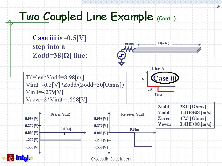
Two Coupled Line Example Case iii is -0. 5[V] step into a Zodd=38[W] line: 10 (Cont. . ) 50[inches] 30[Ohms] Line A Td=len*Vodd=8. 98[ns] Vinit=-0. 5[V]*Zodd/(Zodd+30[Ohms]) Vinit=-. 279[V] Vrcvr=2*Vinit=-. 558[V] 0. 279[V] 0. 000[V] Driver (odd) -0. 5 Time Receiver (odd) 0. 558[V] 9. 0[ns] 0. 279[V] 0. 000[V] -. 279[V] -. 558[V] Case iii V 9. 0[ns] Crosstalk Calculation Zodd Vodd Zeven Veven 38. 0 [Ohms] 1. 41 E+08 [m/s] 47. 5 [Ohms] 1. 41 E+08 [m/s]

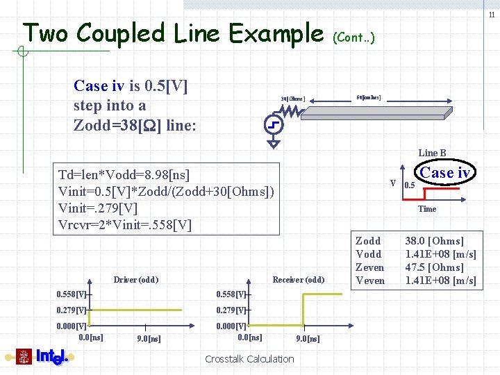
Two Coupled Line Example Case iv is 0. 5[V] step into a Zodd=38[W] line: 30[Ohms] 11 (Cont. . ) 50[inches] Line B Td=len*Vodd=8. 98[ns] Vinit=0. 5[V]*Zodd/(Zodd+30[Ohms]) Vinit=. 279[V] Vrcvr=2*Vinit=. 558[V] Driver (odd) 0. 558[V] 0. 279[V] 0. 000[V] 0. 0[ns] Crosstalk Calculation 0. 5 Case iv Time Receiver (odd) 0. 558[V] 9. 0[ns] V 9. 0[ns] Zodd Vodd Zeven Veven 38. 0 [Ohms] 1. 41 E+08 [m/s] 47. 5 [Ohms] 1. 41 E+08 [m/s]

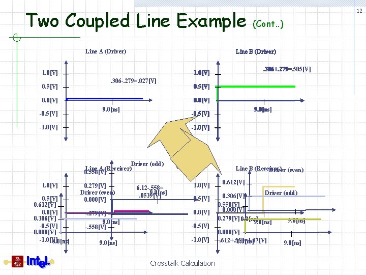
Two Coupled Line Example Line A (Driver) . 306 -. 279=. 027[V] 0. 5[V] 0. 0[V] 9. 0[ns] -1. 0[V] Driver (odd) Line A (Receiver) 0. 558[V] 0. 5[V] 0. 612[V] 0. 0[V] 0. 306[V] -0. 5[V] 0. 000[V] -1. 0[V] 0. 0[ns] 9. 0[ns] -0. 5[V] -1. 0[V] . 306+. 279=. 585[V] 1. 0[V] 0. 0[V] -0. 5[V] (Cont. . ) Line B (Driver) 1. 0[V] 0. 5[V] 12 0. 279[V] Driver (even) 0. 000[V] -. 279[V] 9. 0[ns] -. 558[V] 9. 0[ns] 6. 12 -. 558= 9. 0[ns]. 0539[V] Line B (Receiver) Driver (even) 1. 0[V] 0. 5[V] 0. 0[V] -0. 5[V] -1. 0[V] Crosstalk Calculation 0. 612[V] Driver (odd) 0. 306[V] 0. 558[V] 0. 000[V] 0. 279[V] 0. 0[ns] 9. 0[ns] 0. 000[V]. 612+. 558=1. 17[V] 0. 0[ns] 9. 0[ns]

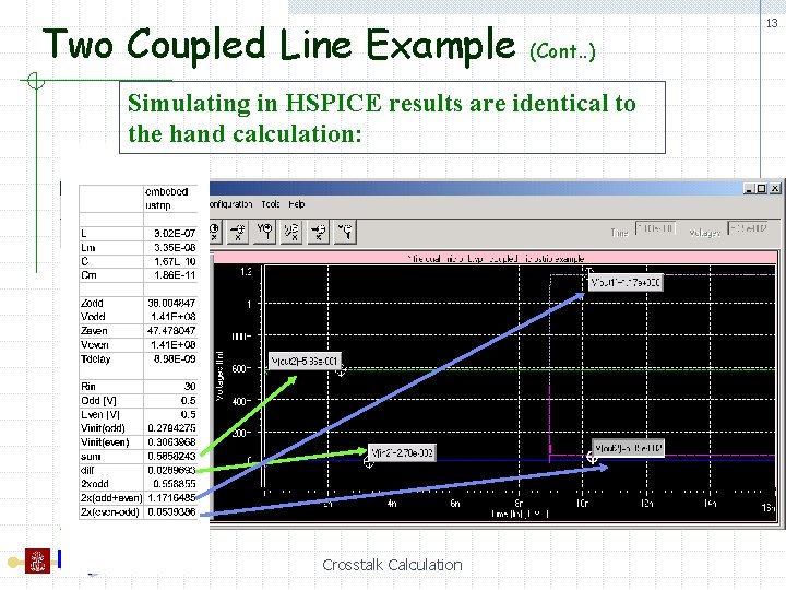
Two Coupled Line Example 13 (Cont. . ) Simulating in HSPICE results are identical to the hand calculation: Crosstalk Calculation

14 Assignment 1 § Use PSPICE and perform previous simulations Crosstalk Calculation

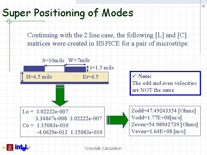
Super Positioning of Modes Continuing with the 2 line case, the following [L] and [C] matrices were created in HSPICE for a pair of microstrips: S=10 mils W=7 mils t=1. 5 mils H=4. 5 mils Er=4. 5 Lo = 3. 02222 e-007 3. 34847 e-008 3. 02222 e-007 Co = 1. 15083 e-010 -4. 0629 e-012 1. 15083 e-010 Crosstalk Calculation ü Note: The odd and even velocities are NOT the same Zodd=47. 49243354 [Ohms] Vodd=1. 77 E+08[m/s] Zeven=54. 98942739 [Ohms] Veven=1. 64 E+08 [m/s] 15

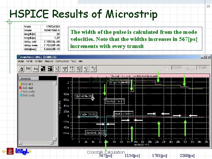
Microstrip Example The solution to this problem follows the same approach as the previous example with one notable difference. The modal velocities are different and result in two different Tdelays: Tdelay (odd)= 7. 19[ns] Tdelay (even)= 7. 75[ns] This means the odd mode voltages will arrive at the end of the line 0. 56[ns] before the even mode voltages Crosstalk Calculation 16

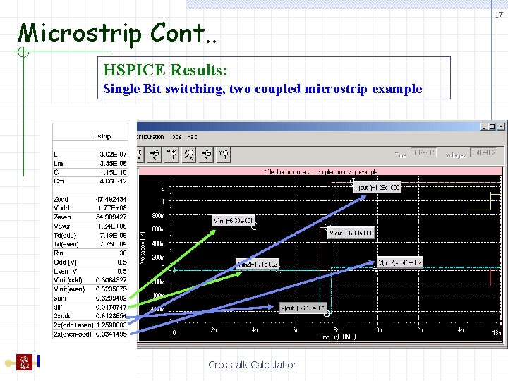
Microstrip Cont. . HSPICE Results: Single Bit switching, two coupled microstrip example Crosstalk Calculation 17

18 HSPICE Results of Microstrip The width of the pulse is calculated from the mode velocities. Note that the widths increases in 567[ps] increments with every transit Calculation Crosstalk Calculation 567[ps] 1134[ps] 1701[ps] 2268[ps]

Assignment 2 and 3 § Use PSPICE and perform previous simulations Crosstalk Calculation 19

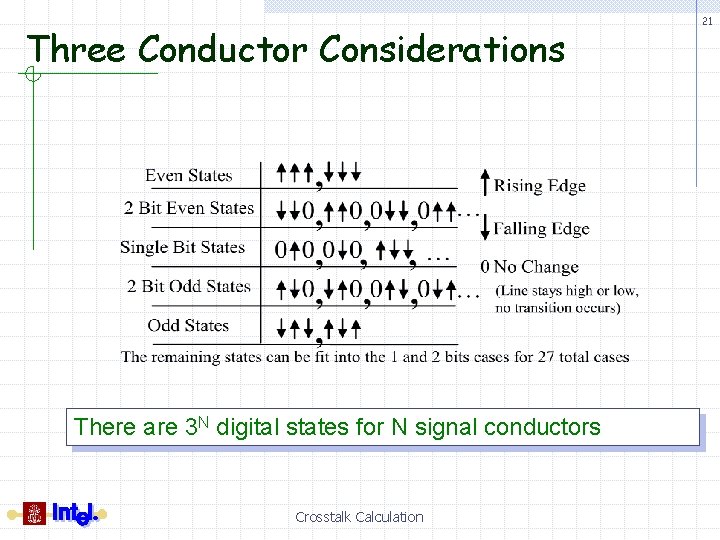
Modal Impedance’s for more than 2 lines § So far we have looked at the two line § crosstalk case, however, most practical busses use more than two lines. Points to Remember: For ‘N’ signal conductors, there are ‘N’ modes. There are 3 N digital states for N signal conductors Each mode has an impedance and velocity associated with it. In homogeneous medium, all the modal velocities will be equal. Any state can be described as a superposition of the modes Crosstalk Calculation 20

Three Conductor Considerations There are 3 N digital states for N signal conductors Crosstalk Calculation 21

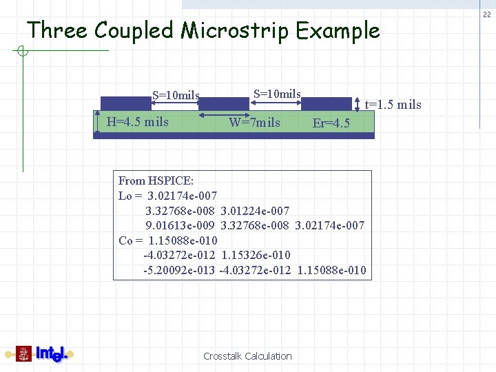
Three Coupled Microstrip Example S=10 mils H=4. 5 mils S=10 mils W=7 mils t=1. 5 mils Er=4. 5 From HSPICE: Lo = 3. 02174 e-007 3. 32768 e-008 3. 01224 e-007 9. 01613 e-009 3. 32768 e-008 3. 02174 e-007 Co = 1. 15088 e-010 -4. 03272 e-012 1. 15326 e-010 -5. 20092 e-013 -4. 03272 e-012 1. 15088 e-010 Crosstalk Calculation 22

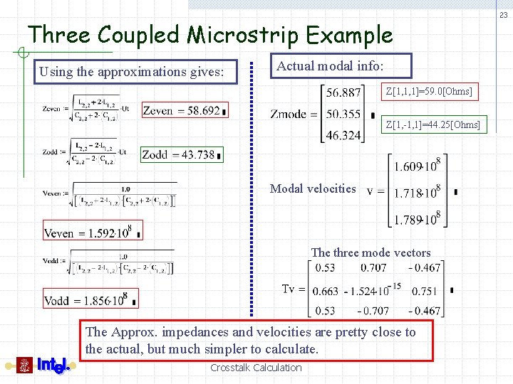
Three Coupled Microstrip Example Using the approximations gives: Actual modal info: Z[1, 1, 1]=59. 0[Ohms] Z[1, -1, 1]=44. 25[Ohms] Modal velocities The three mode vectors The Approx. impedances and velocities are pretty close to the actual, but much simpler to calculate. Crosstalk Calculation 23

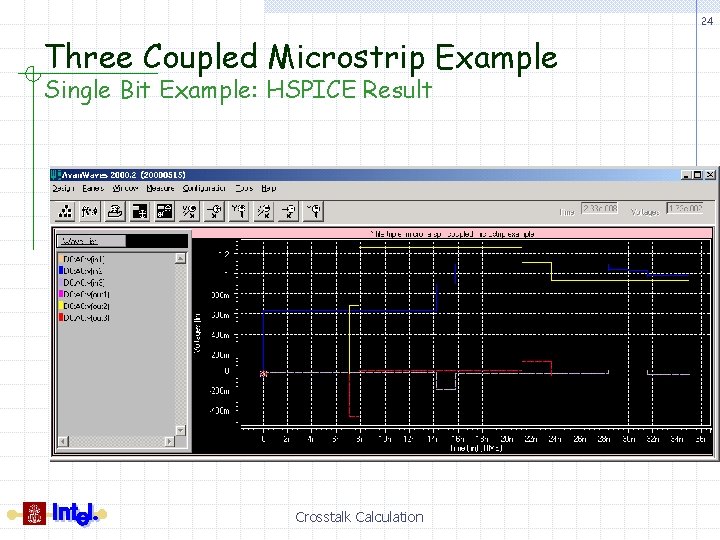
24 Three Coupled Microstrip Example Single Bit Example: HSPICE Result Crosstalk Calculation

Points to Remember § The modal impedances can be used to hand § § § calculate crosstalk waveforms Any state can be described as a superposition of the modes For ‘N’ signal conductors, there are ‘N’ modes. There are 3 N digital states for N signal conductors Each mode has an impedance and velocity associated with it. In homogeneous medium, all the modal velocities will be equal. Crosstalk Calculation 25

Crosstalk Trends Key Topics: üImpedance vs. Spacing üSLEM üTrading Off Tolerance vs. Spacing Crosstalk Calculation 26

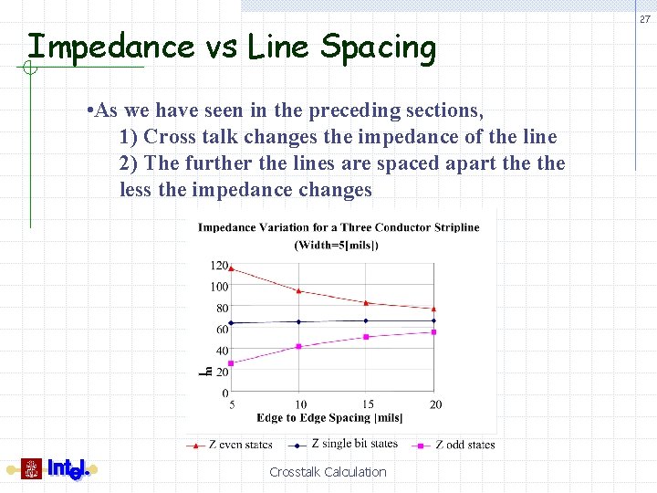
Impedance vs Line Spacing • As we have seen in the preceding sections, 1) Cross talk changes the impedance of the line 2) The further the lines are spaced apart the less the impedance changes Crosstalk Calculation 27

Single Line Equivalent Model 28 (SLEM) § SLEM is an approximation that allows some cross talk effects to be modeled without running fully coupled simulations § Why would we want to avoid fully coupled simulations? Fully coupled simulations tend to be time consuming and dependent on many assumptions Crosstalk Calculation

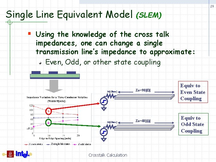
Single Line Equivalent Model 29 (SLEM) § Using the knowledge of the cross talk impedances, one can change a single transmission line’s impedance to approximate: Even, Odd, or other state coupling 30[Ohms] Zo=90[W] 30[Ohms] Zo=40[W] Crosstalk Calculation Equiv to Even State Coupling Equiv to Odd State Coupling

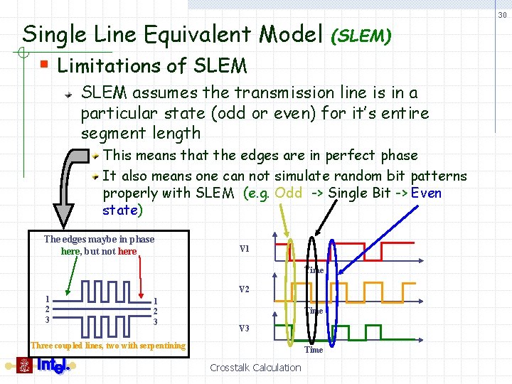
Single Line Equivalent Model 30 (SLEM) § Limitations of SLEM assumes the transmission line is in a particular state (odd or even) for it’s entire segment length This means that the edges are in perfect phase It also means one can not simulate random bit patterns properly with SLEM (e. g. Odd -> Single Bit -> Even state) The edges maybe in phase here, but not here V 1 Time V 2 1 2 3 Time V 3 Three coupled lines, two with serpentining Time Crosstalk Calculation

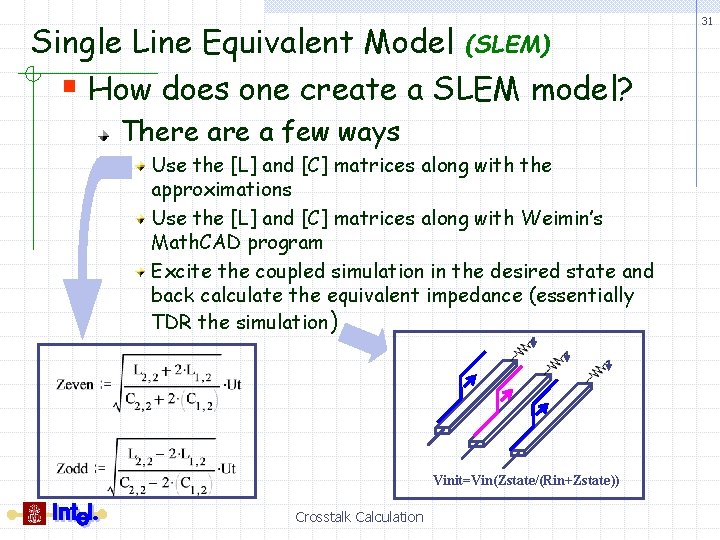
Single Line Equivalent Model (SLEM) § How does one create a SLEM model? There a few ways Use the [L] and [C] matrices along with the approximations Use the [L] and [C] matrices along with Weimin’s Math. CAD program Excite the coupled simulation in the desired state and back calculate the equivalent impedance (essentially TDR the simulation) Vinit=Vin(Zstate/(Rin+Zstate)) Crosstalk Calculation 31

Trading Off Tolerance vs. Spacing § Ultimately in a design you have to create guidelines specifying the trace spacing and specifying the tolerance of the motherboard impedance i. e. 10[mil] edge to edge spacing with 10% impedance variation § Thinking about the spacing in terms of impedance makes this much simpler Crosstalk Calculation 32

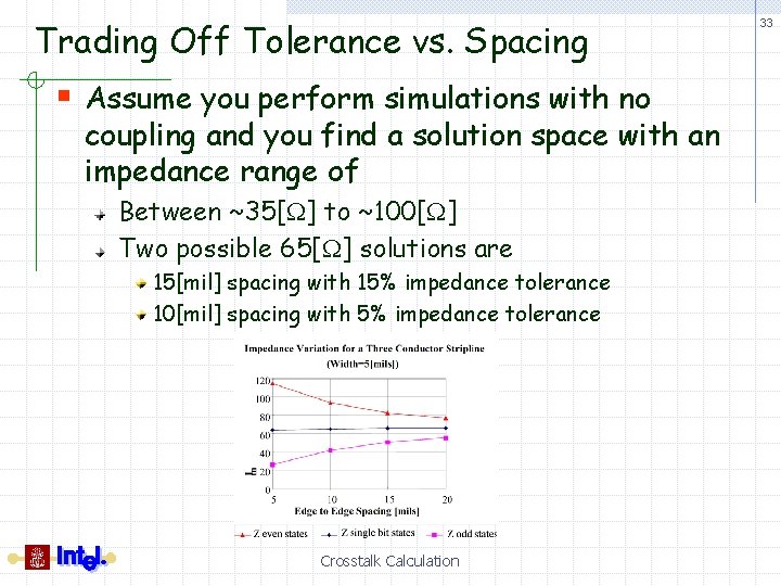
Trading Off Tolerance vs. Spacing § Assume you perform simulations with no coupling and you find a solution space with an impedance range of Between ~35[W] to ~100[W] Two possible 65[W] solutions are 15[mil] spacing with 15% impedance tolerance 10[mil] spacing with 5% impedance tolerance Crosstalk Calculation 33

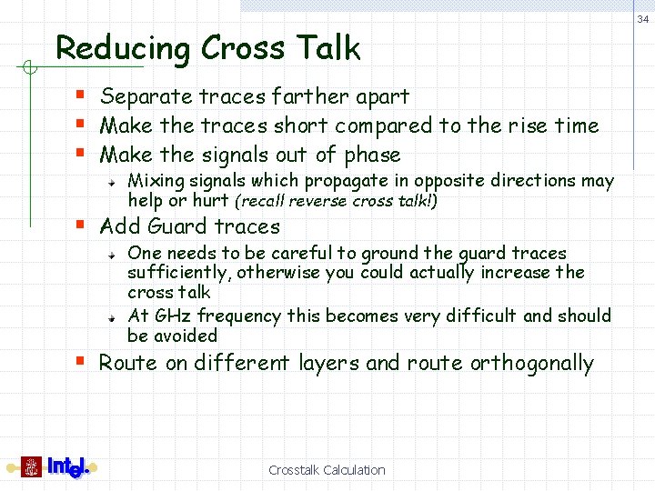
Reducing Cross Talk § Separate traces farther apart § Make the traces short compared to the rise time § Make the signals out of phase Mixing signals which propagate in opposite directions may help or hurt (recall reverse cross talk!) § Add Guard traces One needs to be careful to ground the guard traces sufficiently, otherwise you could actually increase the cross talk At GHz frequency this becomes very difficult and should be avoided § Route on different layers and route orthogonally Crosstalk Calculation 34

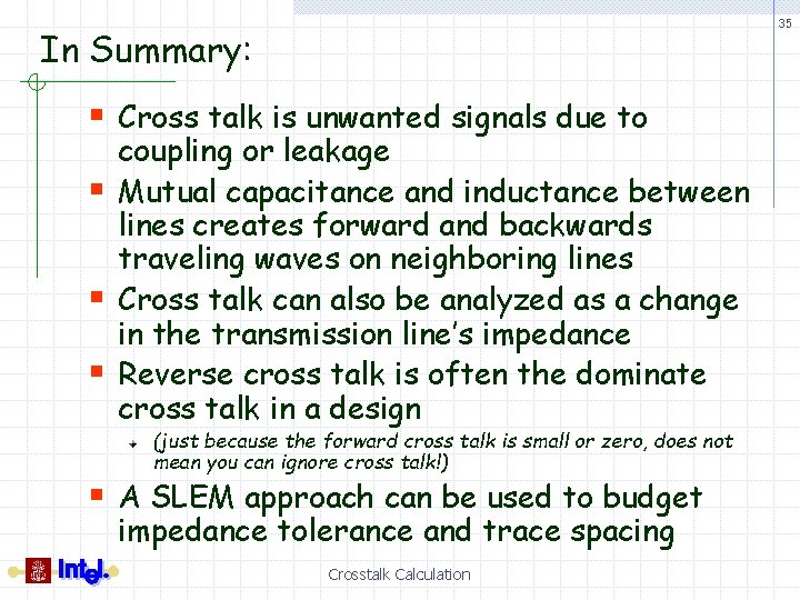
35 In Summary: § Cross talk is unwanted signals due to § § § coupling or leakage Mutual capacitance and inductance between lines creates forward and backwards traveling waves on neighboring lines Cross talk can also be analyzed as a change in the transmission line’s impedance Reverse cross talk is often the dominate cross talk in a design (just because the forward cross talk is small or zero, does not mean you can ignore cross talk!) § A SLEM approach can be used to budget impedance tolerance and trace spacing Crosstalk Calculation