Consumption Saving and Investment Mr Vaughan Income and

Consumption, Saving, and Investment Mr. Vaughan Income and Employment Theory (402) 1

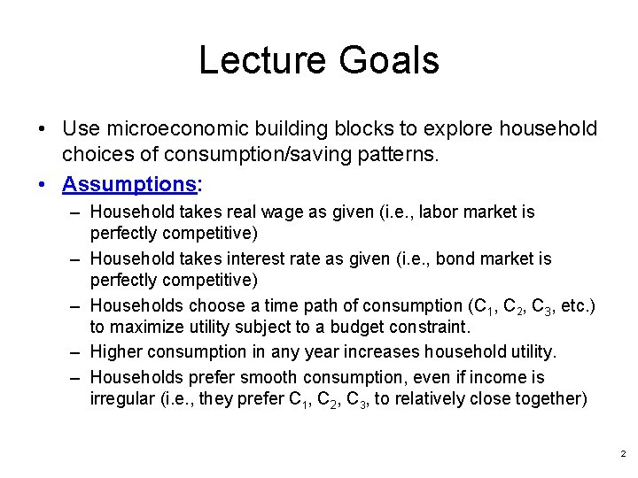
Lecture Goals • Use microeconomic building blocks to explore household choices of consumption/saving patterns. • Assumptions: – Household takes real wage as given (i. e. , labor market is perfectly competitive) – Household takes interest rate as given (i. e. , bond market is perfectly competitive) – Households choose a time path of consumption (C 1, C 2, C 3, etc. ) to maximize utility subject to a budget constraint. – Higher consumption in any year increases household utility. – Households prefer smooth consumption, even if income is irregular (i. e. , they prefer C 1, C 2, C 3, to relatively close together) 2

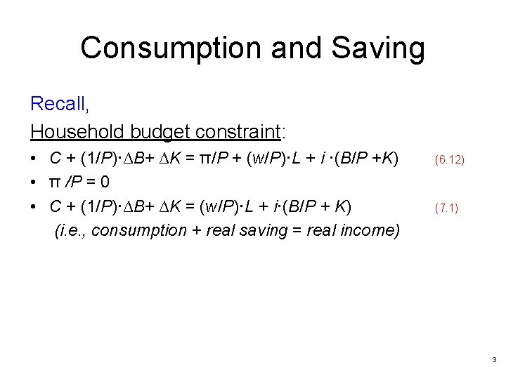
Consumption and Saving Recall, Household budget constraint: • C + (1/P)·∆B+ ∆K = π/P + (w/P)·L + i ·(B/P +K) • π /P = 0 • C + (1/P)·∆B+ ∆K = (w/P)·L + i·(B/P + K) (i. e. , consumption + real saving = real income) (6. 12) (7. 1) 3

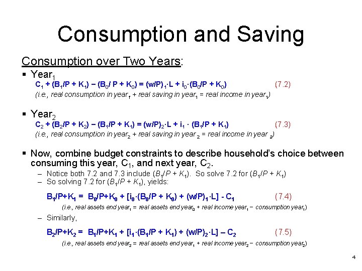
Consumption and Saving Consumption over Two Years: § Year 1 C 1 + (B 1/P + K 1) − (B 0/ P + K 0) = (w/P)1·L + i 0·(B 0/P + K 0) (7. 2) (i. e. , real consumption in year 1 + real saving in year 1 = real income in year 1) § Year 2 C 2 + (B 2/P + K 2) − (B 1/P + K 1) = (w/P)2·L + i 1 · (B 1/P + K 1) (7. 3) (i. e. , real consumption in year 2 + real saving in year 2 = real income in year 2) § Now, combine budget constraints to describe household’s choice between consuming this year, C 1, and next year, C 2. – Notice both 7. 2 and 7. 3 include (B 1/P + K 1). So solve 7. 2 for (B 1/P + K 1) – So solving 7. 2 for (B 1/P + K 1), yields: B 1/P+K 1 = B 0/P+K 0 + [i 0·(B 0/P + K 0) + (w/P)1·L] - C 1 (7. 4) (i. e. , real assets end year 1 = real assets end year 0 + real income year 1 − consumption year 1) – Similarly, B 2/P+K 2 = B 1/P+K 1 + [i 1·(B 1/P + K 1) + (w/P)2·L] – C 2 (7. 5) (i. e. , real assets end year 2 = real assets end year 1 + real income year 2 − consumption year 2) 4

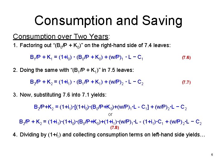
Consumption and Saving Consumption over Two Years: 1. Factoring out “(B 0/P + K 0)” on the right-hand side of 7. 4 leaves: B 1/P + K 1 = (1+i 0) · (B 0/P + K 0) + (w/P)1 · L − C 1 (7. 6) 2. Doing the same with “(B 1/P + K 1)” in 7. 5 leaves: B 2/P + K 2 = (1+i 1) · (B 1/P + K 1) + (w/P)2 · L − C 2 (7. 7) 3. Now, substituting 7. 6 into 7. 1 yields: B 2/P+K 2 = (1+i 1)·[(1+i 0)·(B 0/P+K 0)+(w/P)1·L - C 1] + (w/P)2·L − C 2 or B 2/P + K 2 = (1+i 1)·(1+i 0)·(B 0/P+K 0)+(1+i 1)·(w/P)1·L - (1+i 1)·C 1 + (w/P)2·L − C 2 (7. 8) 4. Dividing by (1+i 1) and collecting consumption terms on left-hand side yields… 5

Consumption and Saving Key Equation (two-year household budget constraint): C 1+[C 2/(1+i 1)] = (1+i 0)·(B 0/P+K 0)+(w/P)1·L + [(w/P)2·L]/(1+i 1) - (B 2/P+K 2)/(1+i 1) (7. 9) § In words: Present value of consumption = Value of initial assets + Present value of of wage incomes − Present value of assets end year 2 § Now, to simplify analysis algebraically, let: V = ( 1 + i 0)·(B 0/P+K 0) + (w/P)1·L + (w/P)2·L/(1+i 1) (7. 10) Present value of sources of funds = Value of initial assets + Present value of wage incomes § So, (7. 9) can be rewritten: C 1+[C 2/(1+i 1)] = V - (B 2/P+K 2)/(1+i 1) (7. 11) Present value of consumption = Present value of initial assets − Present value of assets end year 2 6

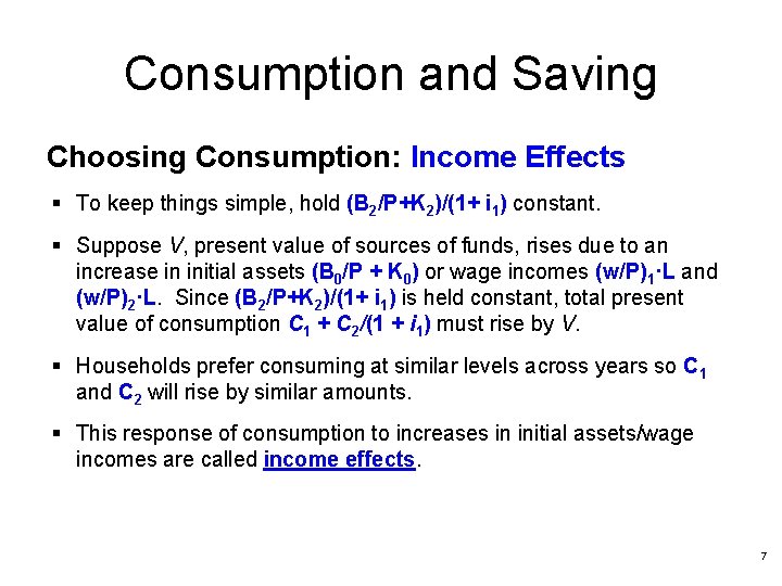
Consumption and Saving Choosing Consumption: Income Effects § To keep things simple, hold (B 2/P+K 2)/(1+ i 1) constant. § Suppose V, present value of sources of funds, rises due to an increase in initial assets (B 0/P + K 0) or wage incomes (w/P)1·L and (w/P)2·L. Since (B 2/P+K 2)/(1+ i 1) is held constant, total present value of consumption C 1 + C 2/(1 + i 1) must rise by V. § Households prefer consuming at similar levels across years so C 1 and C 2 will rise by similar amounts. § This response of consumption to increases in initial assets/wage incomes are called income effects. 7

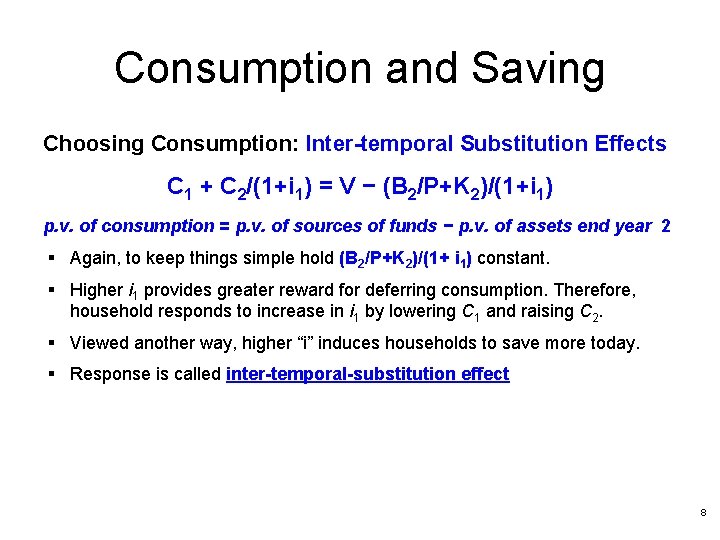
Consumption and Saving Choosing Consumption: Inter-temporal Substitution Effects C 1 + C 2/(1+i 1) = V − (B 2/P+K 2)/(1+i 1) p. v. of consumption = p. v. of sources of funds − p. v. of assets end year 2 § Again, to keep things simple hold (B 2/P+K 2)/(1+ i 1) constant. § Higher i 1 provides greater reward for deferring consumption. Therefore, household responds to increase in i 1 by lowering C 1 and raising C 2. § Viewed another way, higher “i” induces households to save more today. § Response is called inter-temporal-substitution effect 8

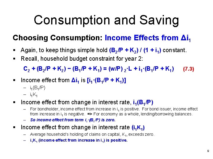
Consumption and Saving Choosing Consumption: Income Effects from Δi 1 § Again, to keep things simple hold (B 2/P + K 2) / (1 + i 1) constant. § Recall, household budget constraint for year 2: C 2 + (B 2/P + K 2) − (B 1/P + K 1) = (w/P) 2·L + i 1·(B 1/P + K 1) (7. 3) § Income effect from Δi 1 is [i 1·(B 1/P + K 1)] – i 1(B 1/P) – i 1 K 1 § Income effect from change in interest rate, i 1(B 1/P) – For bondholder, income effect from increase in i 1 is positive. For bond issuer, income effect from increase in i 1 is negative. => For economy as a whole, lending/borrowing balances. – So income effect from term i 1·(B 1/P) is zero. § Income effect from change in interest rate (i 1 K 1) – Average household’s holding of claims on capital, K 1, exceeds zero. – i 1 K 1 (income effect from increase in i 1) is positive. 9

Consumption and Saving Income effect from change in interest rate § In aggregate, income effect from increase in i 1 consists of zero effect from i 1·(B 1/P) and positive effect from i 1 K 1. § Result: Full income effect from increase in i 1 is positive. 10

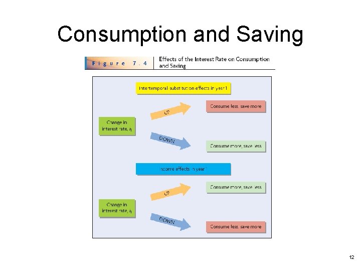
Consumption and Saving Combining Income and Substitution Effects: Effect of increase in current interest rate (i 1) on year 1 consumption (C 1) § Inter-temporal substitution effect motivates household to reduce consumption today (C 1 ↓). § Positive income effect motivates household to raise consumption today (C 1 ↑). § Overall impact on current consumption is ambiguous (C 1 ? ). 11

Consumption and Saving 12

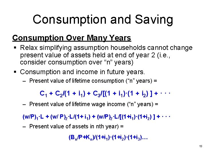
Consumption and Saving Consumption Over Many Years § Relax simplifying assumption households cannot change present value of assets held at end of year 2 (i. e. , consider consumption over “n” years) § Consumption and income in future years. – Present value of lifetime consumption (“n” years) = C 1 + C 2/(1 + i 1) + C 3/[(1 + i 1)·(1 + i 2) ] + · · · – Present value of lifetime wage income (“n” years) = (w/P)1·L + (w/ P)2·L/(1+ i 1) + (w/P)2·L/[(1+i 1)·(1+i 2) ] + · · · – Present value of assets in nth year) = (Bn/P+Kn)/(1+i 1)·(1+i 2)·(1+i 3)… 13

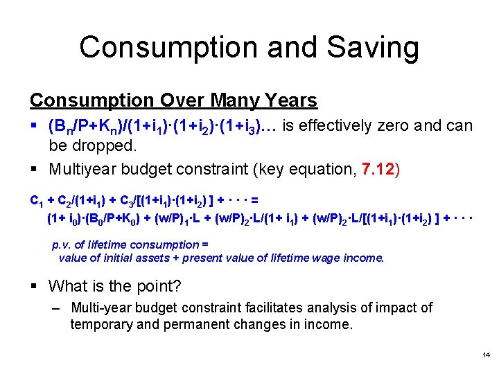
Consumption and Saving Consumption Over Many Years § (Bn/P+Kn)/(1+i 1)·(1+i 2)·(1+i 3)… is effectively zero and can be dropped. § Multiyear budget constraint (key equation, 7. 12) C 1 + C 2/(1+i 1) + C 3/[(1+i 1)·(1+i 2) ] + · · · = (1+ i 0)·(B 0/P+K 0) + (w/P)1·L + (w/P)2·L/(1+ i 1) + (w/P)2·L/[(1+i 1)·(1+i 2) ] + · · · p. v. of lifetime consumption = value of initial assets + present value of lifetime wage income. § What is the point? – Multi-year budget constraint facilitates analysis of impact of temporary and permanent changes in income. 14

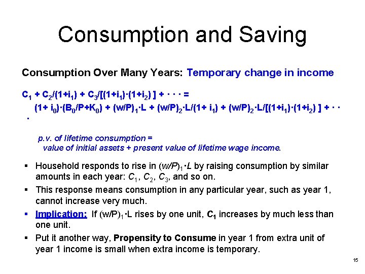
Consumption and Saving Consumption Over Many Years: Temporary change in income C 1 + C 2/(1+i 1) + C 3/[(1+i 1)·(1+i 2) ] + · · · = (1+ i 0)·(B 0/P+K 0) + (w/P)1·L + (w/P)2·L/(1+ i 1) + (w/P)2·L/[(1+i 1)·(1+i 2) ] + · · · p. v. of lifetime consumption = value of initial assets + present value of lifetime wage income. § Household responds to rise in (w/P)1·L by raising consumption by similar amounts in each year: C 1, C 2, C 3, and so on. § This response means consumption in any particular year, such as year 1, cannot increase very much. § Implication: If (w/P)1·L rises by one unit, C 1 increases by much less than one unit. § Put it another way, Propensity to Consume in year 1 from extra unit of year 1 income is small when extra income is temporary. 15

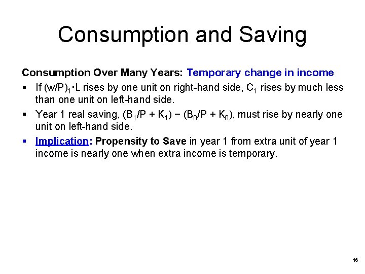
Consumption and Saving Consumption Over Many Years: Temporary change in income § If (w/P)1·L rises by one unit on right-hand side, C 1 rises by much less than one unit on left-hand side. § Year 1 real saving, (B 1/P + K 1) − (B 0/P + K 0), must rise by nearly one unit on left-hand side. § Implication: Propensity to Save in year 1 from extra unit of year 1 income is nearly one when extra income is temporary. 16

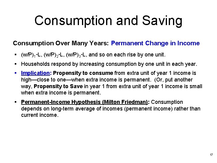
Consumption and Saving Consumption Over Many Years: Permanent Change in Income § (w/P)1·L, (w/P)2·L, (w/P)3·L, and so on each rise by one unit. § Households respond by increasing consumption by one unit in each year. § Implication: Propensity to consume from extra unit of year 1 income is high—close to one—when extra income is permanent. (Or, put another way, Propensity to Save in year 1 from extra unit of year 1 income is small when extra income is permanent. § Permanent-Income Hypothesis (Milton Friedman): Consumption depends on long-term average of incomes (permanent income) rather than current income. 17

Consumption, Saving, and Investment in Equilibrium • Determine aggregate quantities of consumption and saving. • Determine aggregate quantity of investment. 18

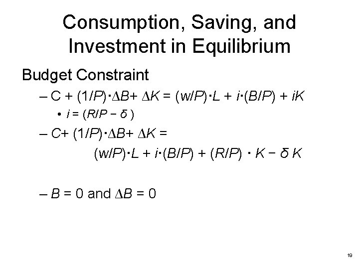
Consumption, Saving, and Investment in Equilibrium Budget Constraint – C + (1/P)·∆B+ ∆K = (w/P)·L + i·(B/P) + i. K • i = (R/P − δ ) – C+ (1/P)·∆B+ ∆K = (w/P)·L + i·(B/P) + (R/P) · K − δ K – B = 0 and ∆B = 0 19

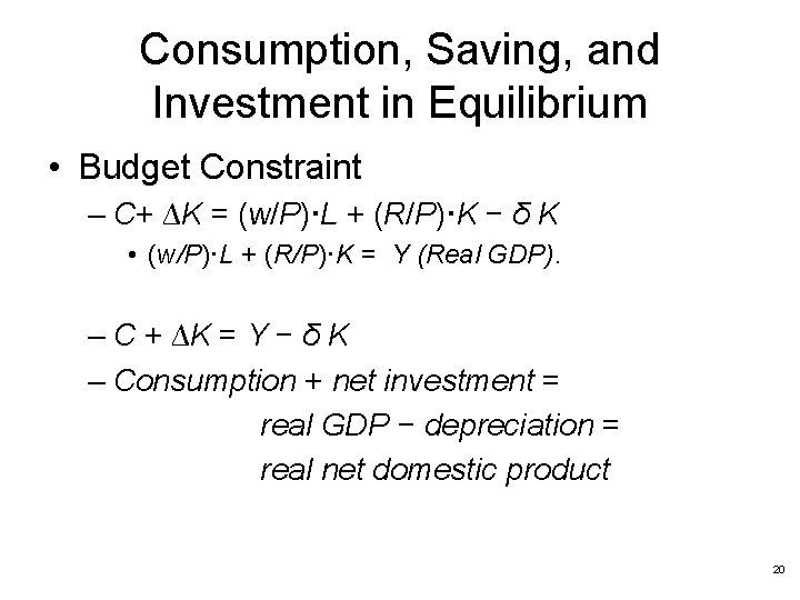
Consumption, Saving, and Investment in Equilibrium • Budget Constraint – C+ ∆K = (w/P)·L + (R/P)·K − δ K • (w/P)·L + (R/P)·K = Y (Real GDP). – C + ∆K = Y − δ K – Consumption + net investment = real GDP − depreciation = real net domestic product 20

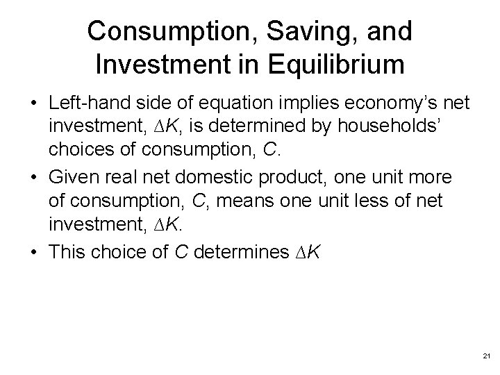
Consumption, Saving, and Investment in Equilibrium • Left-hand side of equation implies economy’s net investment, ∆K, is determined by households’ choices of consumption, C. • Given real net domestic product, one unit more of consumption, C, means one unit less of net investment, ∆K. • This choice of C determines ∆K 21