Consumer Theory Demand Dr Jennifer P Wissink 2011

Consumer Theory Demand Dr. Jennifer P. Wissink © 2011 John M. Abowd and Jennifer P. Wissink, all rights reserved.

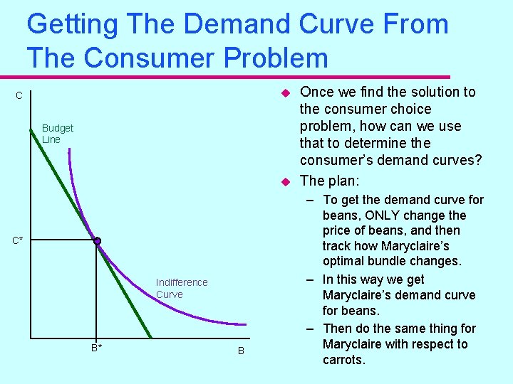
Getting The Demand Curve From The Consumer Problem u C Budget Line u C* Indifference Curve B* B Once we find the solution to the consumer choice problem, how can we use that to determine the consumer’s demand curves? The plan: – To get the demand curve for beans, ONLY change the price of beans, and then track how Maryclaire’s optimal bundle changes. – In this way we get Maryclaire’s demand curve for beans. – Then do the same thing for Maryclaire with respect to carrots.

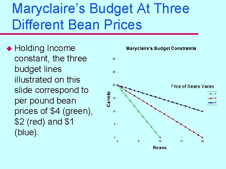
Maryclaire’s Budget At Three Different Bean Prices u Holding Income constant, the three budget lines illustrated on this slide correspond to per pound bean prices of $4 (green), $2 (red) and $1 (blue).

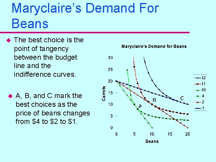
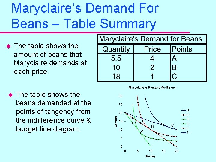
Maryclaire’s Demand For Beans u u The best choice is the point of tangency between the budget line and the indifference curves. A, B, and C mark the best choices as the price of beans changes from $4 to $2 to $1.

Maryclaire’s Demand For Beans – Table Summary u u The table shows the amount of beans that Maryclaire demands at each price. The table shows the beans demanded at the points of tangency from the indifference curve & budget line diagram.

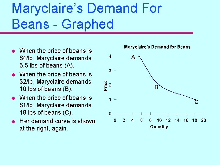
Maryclaire’s Demand For Beans - Graphed u u When the price of beans is $4/lb, Maryclaire demands 5. 5 lbs of beans (A). When the price of beans is $2/lb, Maryclaire demands 10 lbs of beans (B). When the price of beans is $1/lb, Maryclaire demands 18 lbs of beans (C). Her demand curve is shown at the right, again.

The Law Of Demand: Total, Substitution & Income Effects u Question: Will a demand curve ALWAYS be downward sloping? u Economists decompose the total effect of a change in price on the quantity demanded into an income and a substitution effect. u Income effect: due to the increase in real income associated with a fall in prices (you can buy more with the same nominal income) or the loss of real income associated with a rise in prices (you cannot buy as much as you once did with the same nominal income). u Substitution effect: due to the change in the relative price of the good, cheaper goods are substituted for more expensive ones.

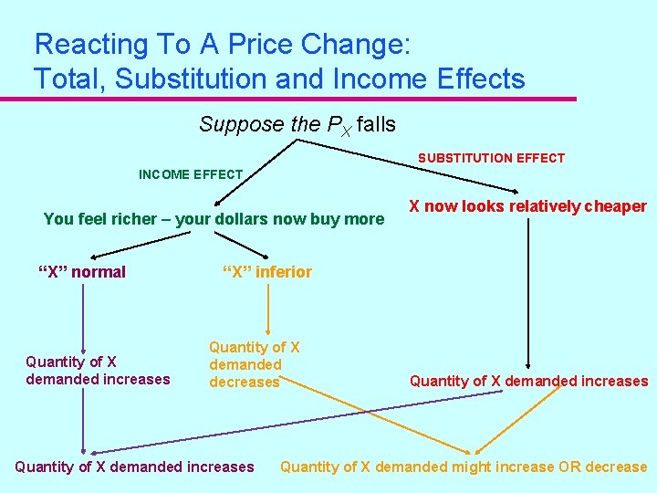
Reacting To A Price Change: Total, Substitution and Income Effects Suppose the PX falls SUBSTITUTION EFFECT INCOME EFFECT You feel richer – your dollars now buy more “X” normal Quantity of X demanded increases X now looks relatively cheaper “X” inferior Quantity of X demanded decreases Quantity of X demanded increases Quantity of X demanded might increase OR decrease

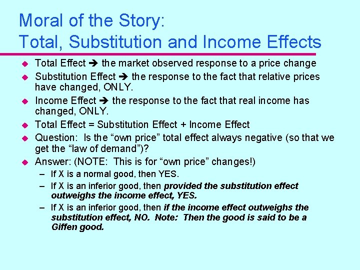
Moral of the Story: Total, Substitution and Income Effects u u u Total Effect the market observed response to a price change Substitution Effect the response to the fact that relative prices have changed, ONLY. Income Effect the response to the fact that real income has changed, ONLY. Total Effect = Substitution Effect + Income Effect Question: Is the “own price” total effect always negative (so that we get the “law of demand”)? Answer: (NOTE: This is for “own price” changes!) – If X is a normal good, then YES. – If X is an inferior good, then provided the substitution effect outweighs the income effect, YES. – If X is an inferior good, then if the income effect outweighs the substitution effect, NO. Note: Then the good is said to be a Giffen good.

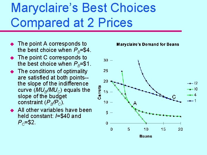
Maryclaire’s Best Choices Compared at 2 Prices u u The point A corresponds to the best choice when PB=$4. The point C corresponds to the best choice when PB=$1. The conditions of optimality are satisfied at both points-the slope of the indifference curve (MUB/MUC) equals the slope of the budget constraint (PB/PC). All other variables have been held constant: I=$40 and PC=$2.

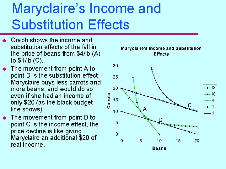
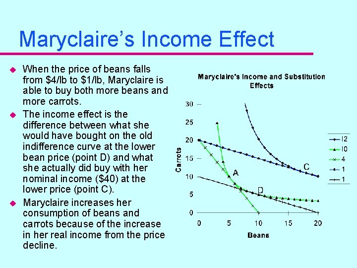
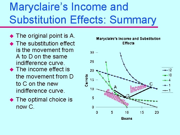
Maryclaire’s Income and Substitution Effects u u u Graph shows the income and substitution effects of the fall in the price of beans from $4/lb (A) to $1/lb (C). The movement from point A to point D is the substitution effect: Maryclaire buys less carrots and more beans, and would do so even if she had an income of only $20 (as the black budget line shows). The movement from point D to point C is the income effect, the price decline is like giving Maryclaire an additional $20 of real income.

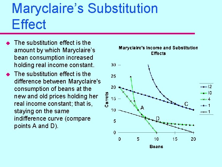
Maryclaire’s Substitution Effect u u The substitution effect is the amount by which Maryclaire’s bean consumption increased holding real income constant. The substitution effect is the difference between Maryclaire's consumption of beans at the new and old prices holding her real income constant; that is, staying on the same indifference curve (compare points A and D).

Maryclaire’s Income Effect u u u When the price of beans falls from $4/lb to $1/lb, Maryclaire is able to buy both more beans and more carrots. The income effect is the difference between what she would have bought on the old indifference curve at the lower bean price (point D) and what she actually did buy with her nominal income ($40) at the lower price (point C). Maryclaire increases her consumption of beans and carrots because of the increase in her real income from the price decline.

Maryclaire’s Income and Substitution Effects: Summary u u The original point is A. The substitution effect is the movement from A to D on the same indifference curve. The income effect is the movement from D to C on the new indifference curve. The optimal choice is now C.

From Individual to Market Demand u Market demand is the sum of all individual demands in the economy. u So what ever happened to Katie? u Let’s bring her back into the story. u She is solving the same consumer theory problem as Maryclaire, except with HER preferences and HER income level, but the SAME market prices for beans and carrots. u The market demand, then, is the sum of the quantities demand by Maryclaire and Katie at each market price.

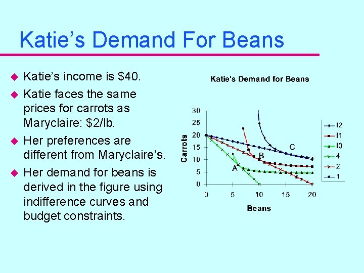
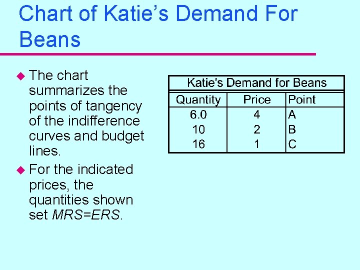
Katie’s Demand For Beans u u Katie’s income is $40. Katie faces the same prices for carrots as Maryclaire: $2/lb. Her preferences are different from Maryclaire’s. Her demand for beans is derived in the figure using indifference curves and budget constraints.

Chart of Katie’s Demand For Beans u The chart summarizes the points of tangency of the indifference curves and budget lines. u For the indicated prices, the quantities shown set MRS=ERS.

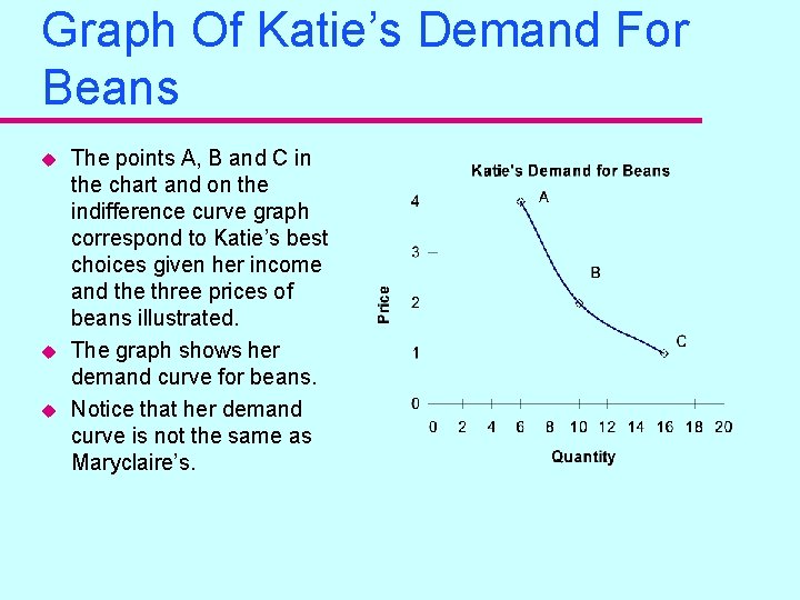
Graph Of Katie’s Demand For Beans u u u The points A, B and C in the chart and on the indifference curve graph correspond to Katie’s best choices given her income and the three prices of beans illustrated. The graph shows her demand curve for beans. Notice that her demand curve is not the same as Maryclaire’s.

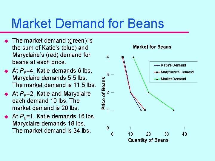
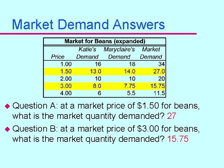
Market Demand for Beans u u The market demand (green) is the sum of Katie’s (blue) and Maryclaire’s (red) demand for beans at each price. At PB=4, Katie demands 6 lbs, Maryclaire demands 5. 5 lbs. The market demand is 11. 5 lbs. At PB=2, Katie and Maryclaire each demand 10 lbs. The market demand is 20 lbs. At PB=1, Katie demands 16 lbs, Maryclaire demands 18 lbs. The market demand is 34 lbs.

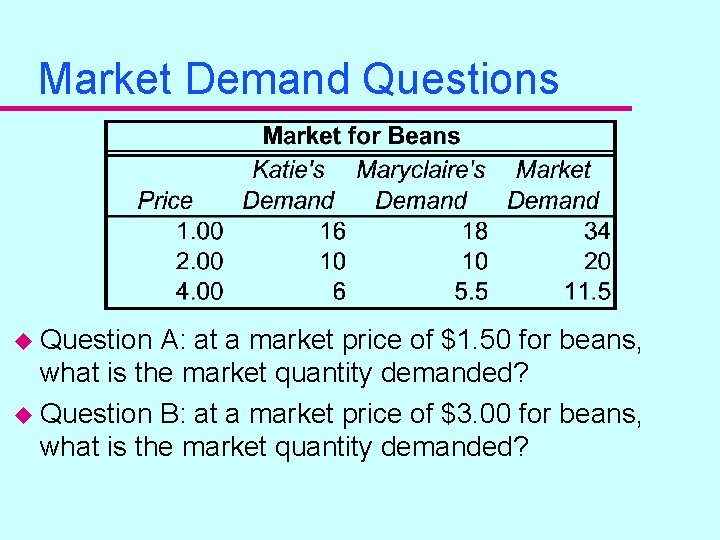
Market Demand Questions u Question A: at a market price of $1. 50 for beans, what is the market quantity demanded? u Question B: at a market price of $3. 00 for beans, what is the market quantity demanded?

Market Demand Answers u Question A: at a market price of $1. 50 for beans, what is the market quantity demanded? 27 u Question B: at a market price of $3. 00 for beans, what is the market quantity demanded? 15. 75

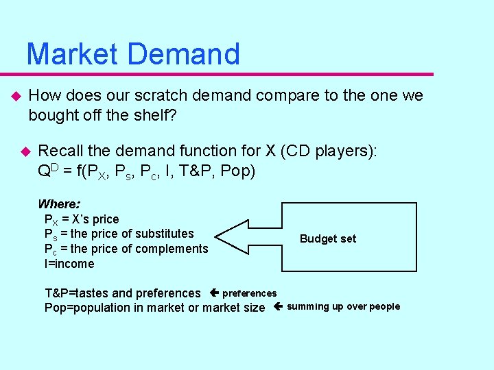
Market Demand u How does our scratch demand compare to the one we bought off the shelf? u Recall the demand function for X (CD players): QD = f(PX, Ps, Pc, I, T&P, Pop) Where: PX = X’s price Ps = the price of substitutes Pc = the price of complements I=income Budget set T&P=tastes and preferences Pop=population in market or market size summing up over people