Equilibrium Applications Lecture 7 Dr Jennifer P Wissink

Announcements-micro Spring 2020 u Prelim 1 is approaching! It is Tuesday March 3. Some suggestions… – Make sure you have at least read through one of the Sample Prelim 1 s that are available via Canvas. Plan to seriously take one of the tests this weekend as a “pretest”. Pretend you are actually taking the prelim and time yourself for 90 minutes. Do as much as you can and then grade yourself. Maybe do this with a friend. And grade each other. Then determine what you need to come and ask the team questions about. Don’t wait until the last minute. – Make sure you look at Prof. Abowd’s Bank of Multiple Choice Questions via Canvas. – Have a peek at Problem Set Files from Wissink SPRING 2003. Good practice there as well! u Hand Written Problem Set 1 is available today! – – – You turn it in at lecture. I will bring a box every time starting Monday. Last lecture to turn it in is Monday March 2. Absolutely no extensions! Answers will be posted immediately after lecture on March 2. If you do it reasonably well and sincerely it counts as 30 My. Econ. Lab points. You are welcomed to work on this with friends and the teaching team.

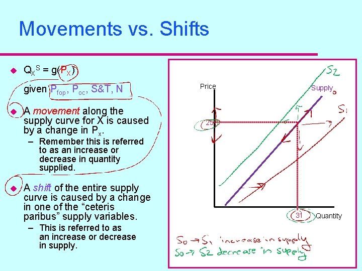
Movements vs. Shifts u QXS = g(PX) given Pfop, Poc, S&T, N u A movement along the supply curve for X is caused by a change in Px. Price Supply 25 – Remember this is referred to as an increase or decrease in quantity supplied. u A shift of the entire supply curve is caused by a change in one of the “ceteris paribus” supply variables. – This is referred to as an increase or decrease in supply. 31 Quantity

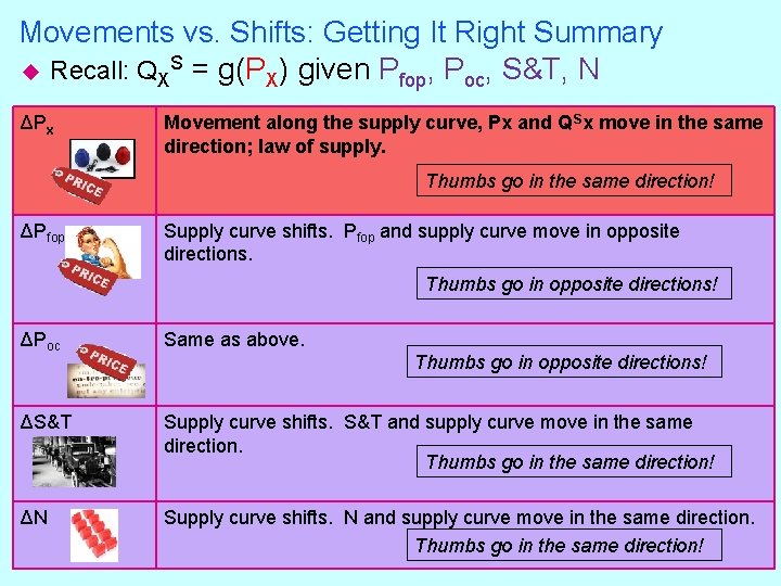
Movements vs. Shifts: Getting It Right Summary u Recall: QXS = g(PX) given Pfop, Poc, S&T, N ΔPx Movement along the supply curve, Px and QSx move in the same direction; law of supply. Thumbs go in the same direction! ΔPfop Supply curve shifts. Pfop and supply curve move in opposite directions. Thumbs go in opposite directions! ΔPoc Same as above. ΔS&T Supply curve shifts. S&T and supply curve move in the same direction. Thumbs go in the same direction! ΔN Supply curve shifts. N and supply curve move in the same direction. Thumbs go in the same direction! Thumbs go in opposite directions!

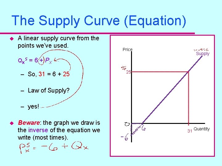
The Supply Curve (Equation) u A linear supply curve from the points we’ve used. Price Supply QXS = 6 + PX – So, 31 = 6 + 25 25 – Law of Supply? – yes! u Beware: the graph we draw is the inverse of the equation we write (most times). 31 Quantity

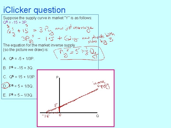
i. Clicker question Suppose the supply curve in market “Y” is as follows: QS = -15 + 3 P. The equation for the market inverse supply (so the picture we draw) is: A. QS = -5 + 1/3 P. B. PS = -15 + 3 Q. C. QS = 15 + 1/3 P. P D. PS = 5 + 1/3 Q. E. PS = 5 – 1/3 Q. Q

Market Equilibrium u We are considering the market for portable speakers. u Recall that we defined the following for our market: – The type and style of portable speakers. – The quality of the portable speakers. – All other attributes of the generic portable speaker. – A time frame that applies to our market for portable speakers. u Demanders are the buyers and from them we get the demand function, etc. – Qx. D = f(PX, Ps, Pc, I, T&P, Pop) u Suppliers are the sellers and from them we get the supply function, etc. – QXS = g(PX, Pfop, Poc, S&T, N) u The market is a perfectly competitive market.

Market Equilibrium (Verbal) u. A place of “rest”. u Equilibrium: a price where the quantity demanded equals the quantity supplied. u In notation: – Find a PX* so that: QXD(PX*) = QXS(PX*)

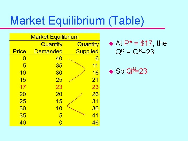
Market Equilibrium (Table) u At P* = $17, the QD = QS=23 u So Q*=23

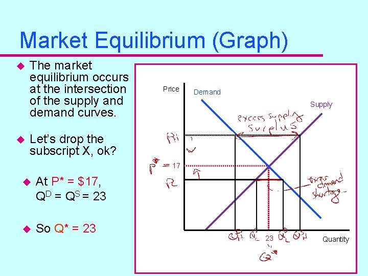
Market Equilibrium (Graph) u u The market equilibrium occurs at the intersection of the supply and demand curves. Price Demand Supply Let’s drop the subscript X, ok? 17 u At P* = $17, QD = QS = 23 u So Q* = 23 23 Quantity

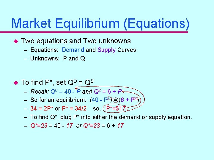
Market Equilibrium (Equations) u Two equations and Two unknowns – Equations: Demand Supply Curves – Unknowns: P and Q u To find P*, set QD = QS – – – Recall: QD = 40 - P and QS = 6 + P So for an equilibrium: (40 - P*) = (6 + P*) 34 = 2 P* or P* = 34/2 so. . . P*=$17 To find Q*, plug P* into either the demand or supply equation. Q*=23 = 40 - 17 or Q*=23 = 6 + 17

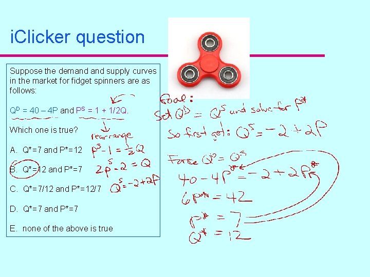
i. Clicker question Suppose the demand supply curves in the market for fidget spinners are as follows: QD = 40 – 4 P and PS = 1 + 1/2 Q. Which one is true? A. Q*=7 and P*=12 B. Q*=12 and P*=7 C. Q*=7/12 and P*=12/7 D. Q*=7 and P*=7 E. none of the above is true

Now What? u u u Comparative Statics! Use the model to make predictions. Something changes in the market. – – u u u Something that changes Demand. Something that changes Supply. Something that changes both! Something the government does to prevent an equilibrium. Would get a new equilibrium. Compare one market equilibrium with another market equilibrium and see what happens to P* and Q*. Compare two equilibriums - compare two static situations comparative statics!

The Roses Market u u What impact does Valentine’s Day have on the roses market in February each year? What do you predict will happen to the equilibrium market price and quantity?

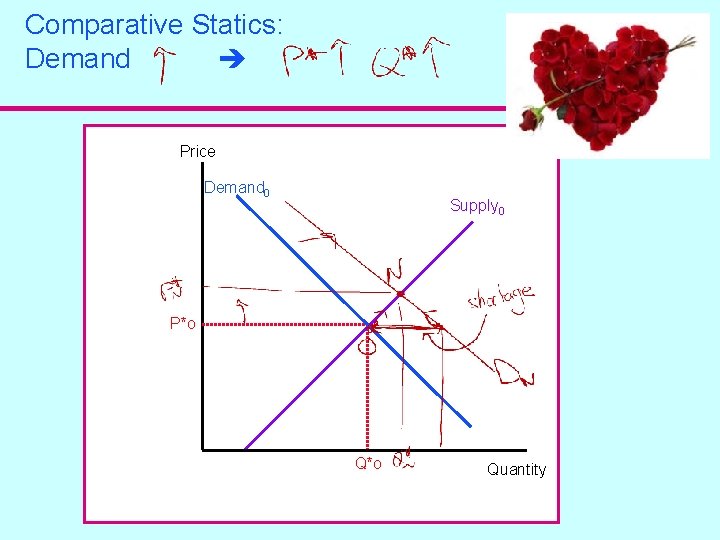
Comparative Statics: Demand Price Demand 0 Supply 0 P*o Quantity

The Oil Market u u u Canadian Court Clears The Way For Trans Mountain Pipeline Expansion https: //www. npr. org/2020/02/05/803002446/canadian-court-clears-theway-for-trans-mountain-pipeline-expansion What do you predict will happen to the equilibrium market price and quantity?

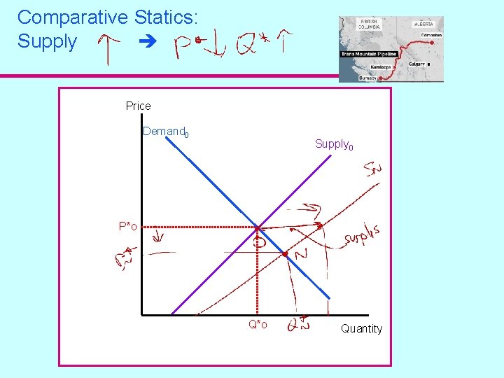
Comparative Statics: Supply Price Demand 0 Supply 0 P*o Quantity

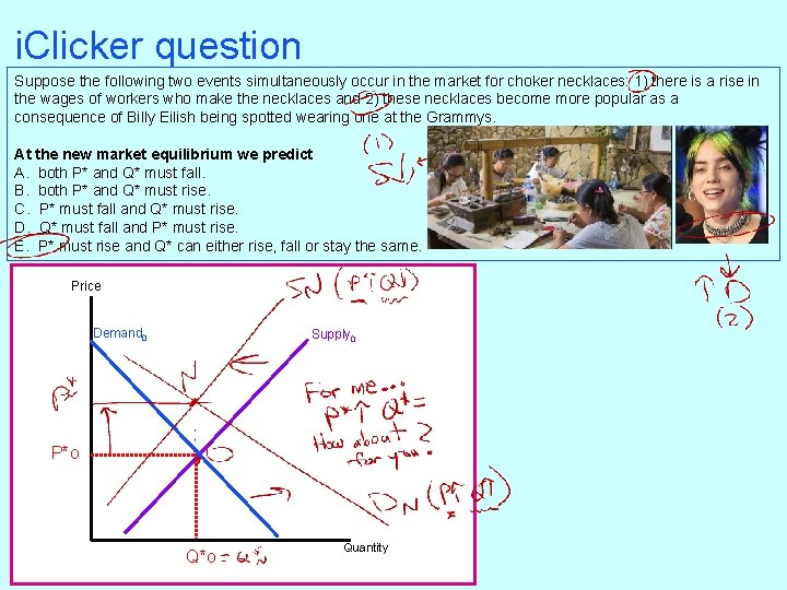
i. Clicker question Suppose the following two events simultaneously occur in the market for choker necklaces: 1) there is a rise in the wages of workers who make the necklaces and 2) these necklaces become more popular as a consequence of Billy Eilish being spotted wearing one at the Grammys. At the new market equilibrium we predict A. both P* and Q* must fall. B. both P* and Q* must rise. C. P* must fall and Q* must rise. D. Q* must fall and P* must rise. E. P* must rise and Q* can either rise, fall or stay the same. Price Demand 0 Supply 0 P*o Quantity

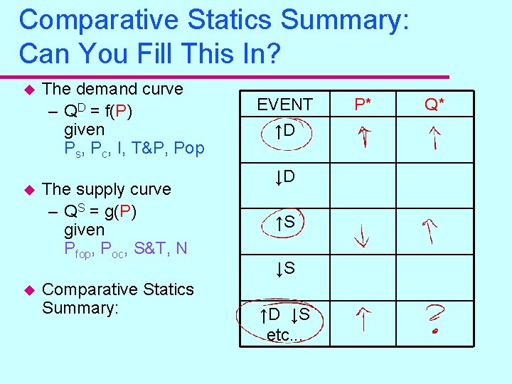
Comparative Statics Summary: Can You Fill This In? u u u The demand curve – QD = f(P) given Ps, Pc, I, T&P, Pop The supply curve – QS = g(P) given Pfop, Poc, S&T, N Comparative Statics Summary: EVENT ↑D ↓D ↑S ↓S ↑D ↓S etc. . . P* Q*

4 Classic Government Interventions u Price Floors u Price Ceilings u Quantity Quotas u Transaction Taxes Ambrogio Lorenzetti, The Effects of Good Government in the city, Siena Italy, circa 1338

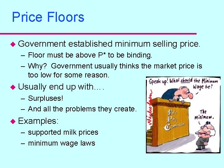
Price Floors u Government established minimum selling price. – Floor must be above P* to be binding. – Why? Government usually thinks the market price is too low for some reason. u Usually end up with…. – Surpluses! – And all the problems they create. u Examples: – supported milk prices – minimum wage laws

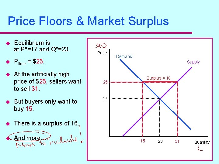
Price Floors & Market Surplus u Equilibrium is at P*=17 and Q*=23. u Pfloor = $25. u At the artificially high price of $25, sellers want to sell 31. u But buyers only want to buy 15. u There is a surplus of 16. u And more… Price Demand Supply Surplus = 16 25 17 15 23 31 Quantity

Price Ceilings u Government established maximum selling price. – Must be below P* to be binding. – Why? Government usually thinks the market price is too high for some reason. u Usually end up with…. – Shortages! – And all the problems they generate. u Examples: – Gas price ceilings – Apartment rent control