Construction of pseudo longitudinal age profiles from crosssectional

Construction of pseudo longitudinal age profiles from cross-sectional NTA estimates Ronald Lee Discussion for Indicators Group June 14, 2010 NTA 7, East West Center, Hawaii

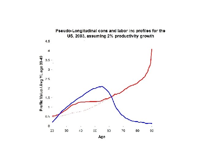
The basic idea • We have an estimate of the cross-sectional profiles, yl(x) and c(x). • Assume that individuals all expect future productivity growth at some rate, let’s say. 015% per year. • For this, you might take an historical average rate of productivity growth or you might borrow the assumption used in official government projections such as by the public pension system. • Then future labor income is expected to be:

• Consumption can be projected in the same way. • Rationale is that the whole economy is expanding at this rate (plus labor force growth rate), so we would expect consumption to as well. • Then ratio of aggregate consumption to aggregate labor income will remain about the same, etc. • It would be possible to make a case for some more complicated approach, and for some purposes you might want an approach with more behavioral theory or with more demography incorporated.

• I did a comparison of the result of this approach to actual longitudinal data for the US, from 1960 to 2003, but I could not find it in my files. • My recollection is that it looked quite good.

Discounting • An individual uses some discount rate for expected future benefits or costs. • There is disagreement about what rate to use. I generally use 3% which is often taken as the “risk free” real interest rate available on US treasury securities. • Some people use higher discount rates, e. g. 5%. • Most of you will know more about this than I do. • Usually it is also appropriate to weight by survival probability.

Discounting (cont. ) • Suppose that public transfers to children are received on average at age 10, and to the elderly at age 70, 60 years later. • Exp(-60*. 03)=. 165, so receiving a dollar when young is worth six dollars when old, which becomes larger after adjusting for survival. Maybe 8 dollars or more, depending on mortality level.

Beckeronia • Tim’s diagram of Prestonia, Disneyland, and Beckeronia showed a slope of 2. 5 for old age benefits versus child benefits, per capita, across countries. • He said this was fair, because of the discounting. • Why shouldn’t the slope be six for fairness in Beckeronia?

Beckeronia (cont. ) • Factor of six comes when we compare the actual dollars received in youth and old age. • But the current cross section only shows the dollars received by kids and elders today. • To get future dollars we have to inflate by. 015 prod gr for 60 years. Then we discount back at 3%. • Same as discounting the cross-section at. 015. • Exp(-60*. 015)=. 40!

For some purposes, we may want to remove cohort specific bumps and trends • Example of problem (1) – The US labor income profile peaks quite late and is relatively high at old ages compared to other countries. – Probably this is due to the history of rising educational attainment in the US. Current elderly have education quite similar to younger workers. – Maybe we would want to take this into account when we project forward, so that this feature of the profile eventually disappears in our projections.

Example (2) • The US public pension system changed the system of indexing benefits to prices and wages a while ago. • They made a mistake and double indexed to inflation. • This means that a few birth cohorts received higher benefits than was intended, the “notch” generations. • This puts a bump in the pension benefit profile.

Example (2) continued • Suppose you have two age profiles of benefits separated by a year or two. • You can calculate the age profile of longitudinal growth rates of pensions as below. • This reflects both productivity growth in the past and normal changes in pensions longitudinally, e. g. due to changing proportions widowed, selectivity of survival, etc. • If this is used instead of the previous method to project forward, adding new initial benefit levels, then the bulge will move to older ages and eventually die out.

The household and aggregate demand for life cycle wealth • Demand for “life cycle wealth” at age x is amount of wealth needed to achieve planned consumption given planned labor income over remaining life. W(x) • Key assumption: adults expect age profiles of labor income and consumption to rise at rate of productivity growth, e. g. 2% per year (used here). • In this example, the consumption of children is folded into the planned consumption of adults, by age of child. So intrahousehold transfers to children are implicit. • This is just the example I was able to find in my files last night; could just as well do this on purely individual basis.

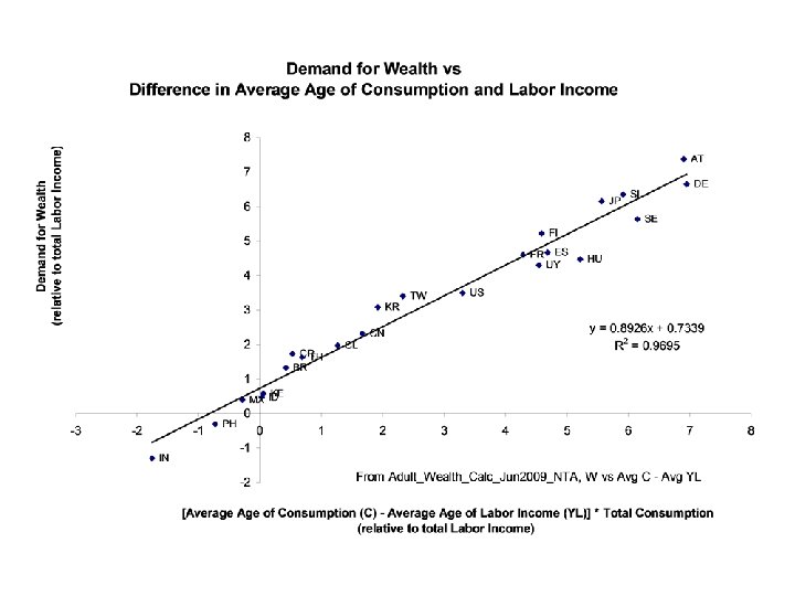
• Using these pseudo-longitudinal profiles we can now calculate the demand for wealth per adult at each age. • We can then calculate the weighted average across the entire adult population, to find the aggregate demand for wealth, W. • A simple measure under the golden rule assumption is given by the Willis Theorem:

• Next slide shows a scatter diagram that compares the numerical calculation based on method I just described to the golden rule analytic result. • Obviously, NTA countries are not golden rule economies. Not in economic steady state, not stable populations, not as deep in capital as golden rule requires.