Computational Discovery of Explanatory Process Models Pat Langley

Computational Discovery of Explanatory Process Models Pat Langley Computational Learning Laboratory Center for the Study of Language and Information Stanford University, Stanford, California http: //cll. stanford. edu/~langley@csli. stanford. edu Thanks to N. Asgharbeygi, K. Arrigo, S. Bay, S. Dzeroski, A. Pohorille, J. Sanchez, K. Saito, Oren Shiran, J. Shrager, and L. Todorovski for their contributions to this research, which is funded by a grant from the National Science Foundation.

Adbuctive Model Construction Most mature sciences focus their efforts not on discovering laws or forming theories, but on constructing models that: · build upon known laws and theoretical principles; · adapt this knowledge to a particular scientific setting; · augment the knowledge with auxiliary assumptions; · use the resulting model to explain observed phenomena. This task involves abduction of explanatory models from domain knowledge, though it may also have inductive aspects. In this talk, I examine the construction of explanatory models for dynamical systems that change over time.

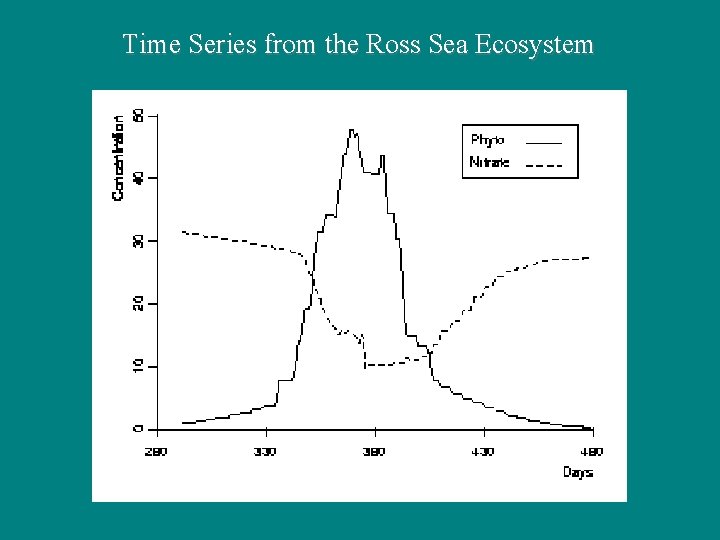
Time Series from the Ross Sea Ecosystem

Inductive Process Modeling Our approach is to design and implement computational methods for inductive process modeling, which: · represent scientific models as sets of quantitative processes; · use these models to predict and explain observational data; · search a space of process models to find good candidates; · utilize background knowledge to constrain this search. This framework has great potential both for modeling scientific reasoning and aiding practicing scientists.

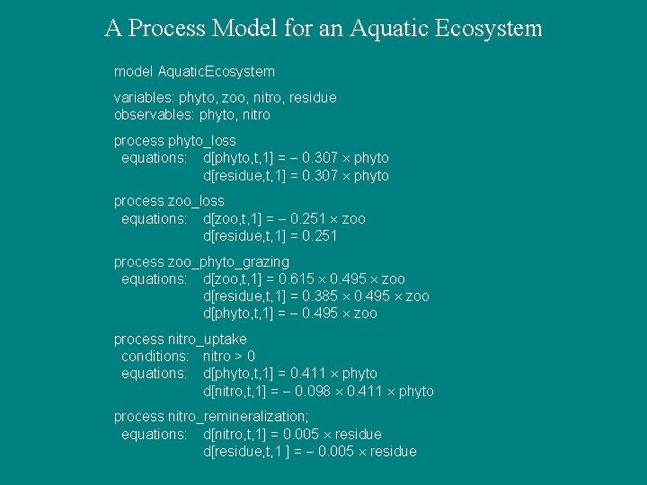
A Process Model for an Aquatic Ecosystem model Aquatic. Ecosystem variables: phyto, zoo, nitro, residue observables: phyto, nitro process phyto_loss equations: d[phyto, t, 1] = 0. 307 phyto d[residue, t, 1] = 0. 307 phyto process zoo_loss equations: d[zoo, t, 1] = 0. 251 zoo d[residue, t, 1] = 0. 251 process zoo_phyto_grazing equations: d[zoo, t, 1] = 0. 615 0. 495 zoo d[residue, t, 1] = 0. 385 0. 495 zoo d[phyto, t, 1] = 0. 495 zoo process nitro_uptake conditions: nitro > 0 equations: d[phyto, t, 1] = 0. 411 phyto d[nitro, t, 1] = 0. 098 0. 411 phyto process nitro_remineralization; equations: d[nitro, t, 1] = 0. 005 residue d[residue, t, 1 ] = 0. 005 residue

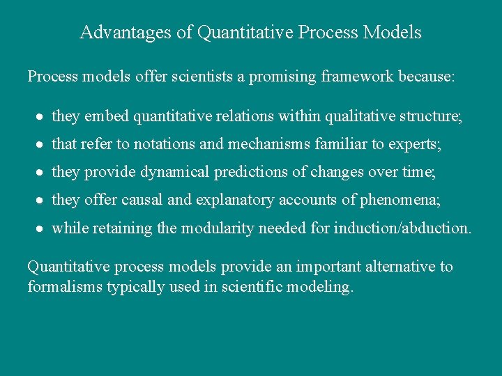
Advantages of Quantitative Process Models Process models offer scientists a promising framework because: · they embed quantitative relations within qualitative structure; · that refer to notations and mechanisms familiar to experts; · they provide dynamical predictions of changes over time; · they offer causal and explanatory accounts of phenomena; · while retaining the modularity needed for induction/abduction. Quantitative process models provide an important alternative to formalisms typically used in scientific modeling.

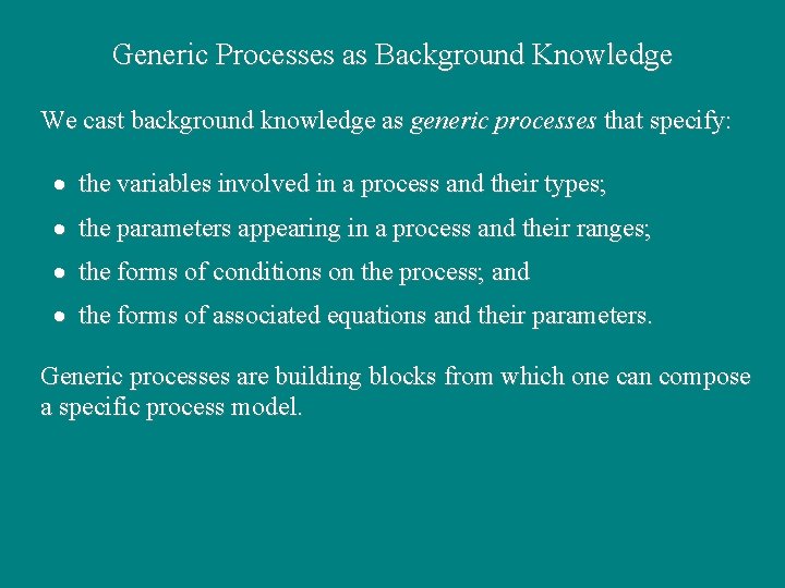
Generic Processes as Background Knowledge We cast background knowledge as generic processes that specify: · the variables involved in a process and their types; · the parameters appearing in a process and their ranges; · the forms of conditions on the process; and · the forms of associated equations and their parameters. Generic processes are building blocks from which one can compose a specific process model.

Generic Processes for Aquatic Ecosystems generic process exponential_loss variables: S{species}, D{detritus} parameters: [0, 1] equations: d[S, t, 1] = 1 S d[D, t, 1] = S generic process remineralization variables: N{nutrient}, D{detritus} parameters: [0, 1] equations: d[N, t, 1] = D d[D, t, 1] = 1 D generic process grazing variables: S 1{species}, S 2{species}, D{detritus} parameters: [0, 1], [0, 1] equations: d[S 1, t, 1] = S 1 d[D, t, 1] = (1 ) S 1 d[S 2, t, 1] = 1 S 1 generic process constant_inflow variables: N{nutrient} parameters: [0, 1] equations: d[N, t, 1] = generic process nutrient_uptake variables: S{species}, N{nutrient} parameters: [0, ], [0, 1] conditions: N > equations: d[S, t, 1] = S d[N, t, 1] = 1 S

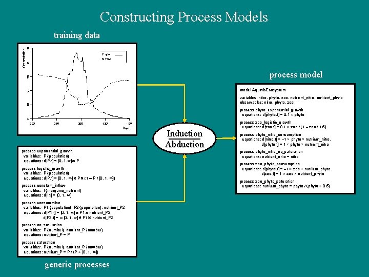
Constructing Process Models training data process model Aquatic. Ecosystem variables: nitro, phyto, zoo, nutrient_nitro, nutrient_phyto observables: nitro, phyto, zoo process phyto_exponential_growth equations: d[phyto, t] = 0. 1 phyto process exponential_growth variables: P {population} equations: d[P, t] = [0, 1, ] P process logistic_growth variables: P {population} equations: d[P, t] = [0, 1, ] P (1 P / [0, 1, ]) process constant_inflow variables: I {inorganic_nutrient} equations: d[I, t] = [0, 1, ] process consumption variables: P 1 {population}, P 2 {population}, nutrient_P 2 equations: d[P 1, t] = [0, 1, ] P 1 nutrient_P 2, d[P 2, t] = [0, 1, ] P 1 nutrient_P 2 process no_saturation variables: P {number}, nutrient_P {number} equations: nutrient_P = P process saturation variables: P {number}, nutrient_P {number} equations: nutrient_P = P / (P + [0, 1, ]) generic processes Induction Abduction process zoo_logistic_growth equations: d[zoo, t] = 0. 1 zoo / (1 zoo / 1. 5) process phyto_nitro_consumption equations: d[nitro, t] = 1 phyto nutrient_nitro, d[phyto, t] = 1 phyto nutrient_nitro process phyto_nitro_no_saturation equations: nutrient_nitro = nitro process zoo_phyto_consumption equations: d[phyto, t] = 1 zoo nutrient_phyto, d[zoo, t] = 1 zoo nutrient_phyto process zoo_phyto_saturation equations: nutrient_phyto = phyto / (phyto + 0. 5)

A Method for Process Model Construction The IPM algorithm constructs explanatory models from generic elements components in four stages: 1. Find all ways to instantiate known generic processes with specific variables, subject to type constraints; 2. Combine instantiated processes into candidate generic models subject to additional constraints (e. g. , number of processes); 3. For each generic model, carry out search through parameter space to find good coefficients; 4. Return the parameterized model with the best overall score. Our typical evaluation metric is squared error, but we have also explored other measures of explanatory adequacy.

Estimating Parameters in Process Models To estimate the parameters for each generic model structure, the IPM algorithm: 1. Selects random initial values that fall within ranges specified in the generic processes; 2. Improves these parameters using the Levenberg-Marquardt method until it reaches a local optimum; 3. Generates new candidate values through random jumps along dimensions of the parameter vector and continue search; 4. If no improvement occurs after N jumps, it restarts the search from a new random initial point. This multi-level method gives reasonable fits to time-series data from a number of domains, but it is computationally intensive.

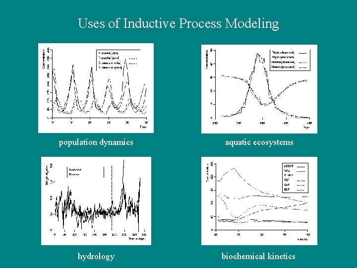
Uses of Inductive Process Modeling population dynamics aquatic ecosystems hydrology biochemical kinetics

Intellectual Influences Our approach to explanatory model construction draws on ideas from many traditions: · computational scientific discovery (e. g. , Todorovski, 2003); · methods for causal model abduction (e. g. , Zupan et al. , 2001); · qualitative physics and simulation (e. g. , Forbus, 1984); · languages for scientific simulation (e. g. , STELLA, MATLAB). Our work combines these ideas in novel ways to support abduction of models that explain the behavior of dynamical systems.

Some Recent Extensions In recent work, we have extended our approach to incorporate: · heuristic beam search through the space of process models; · hierarchical generic processes that further constrain search; · an ensemble-like method that mitigates overfitting effects; · metrics for explanatory adequacy based on trajectory shapes. We have also embedded our algorithms in an interactive software environment for model construction and revision.

End of Presentation

Backup Slides

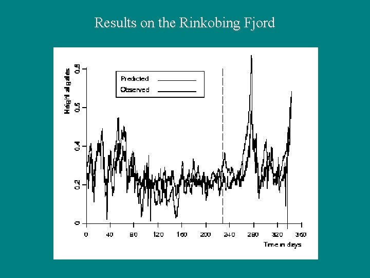
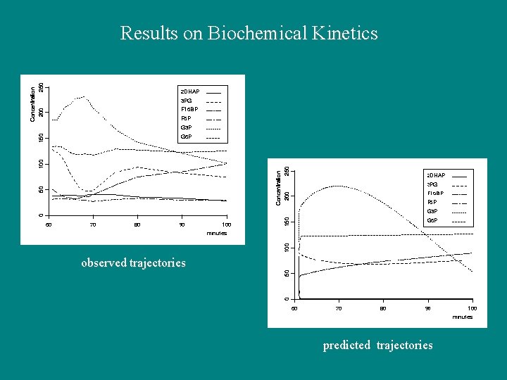
Generating Predictions and Explanations To utilize or evaluate a given process model, we must simulate its behavior over time: · specify initial values for input variables and time step size; · on each time step, determine which processes are active; · solve active algebraic/differential equations with known values; · propagate values and recursively solve other active equations; · when multiple processes influence the same variable, assume their effects are additive. This performance method makes specific predictions that we can compare to observations.

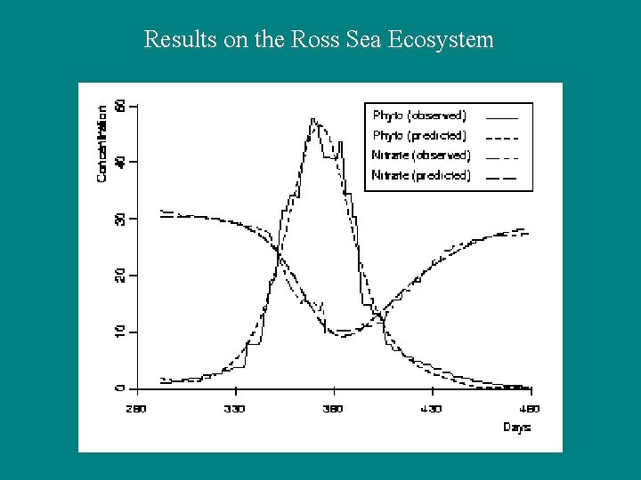
Results on the Ross Sea Ecosystem

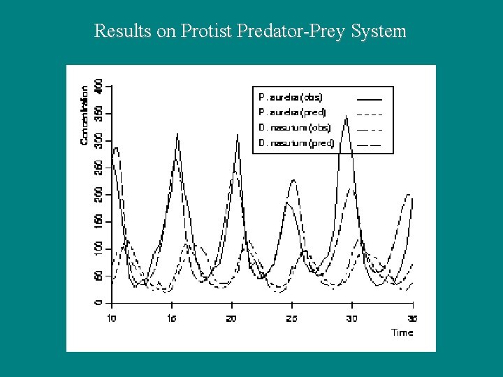
Results on Protist Predator-Prey System

Results on the Rinkobing Fjord

Results on Biochemical Kinetics observed trajectories predicted trajectories