Remove redundant explanatory variables Reexpress explanatory variables Do


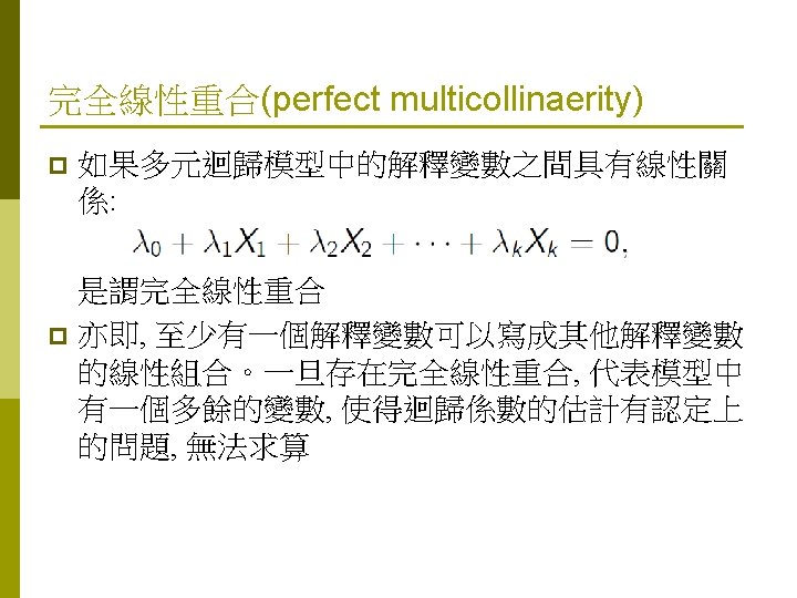
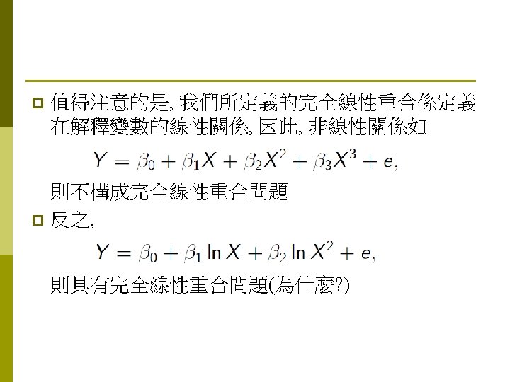


如何解決線性重合問題 § § § Remove redundant explanatory variables. Re-express explanatory variables Do nothing if the explanatory variables are significant with sensible estimates. 26 of 46 Copyright © 2011 Pearson Education, Inc.

Example : RETAIL PROFITS p Motivation p A chain of pharmacies is looking to expand into a new community. It has data for 110 cities on the following variables: income, disposable income, birth rate, social security recipients, cardiovascular deaths and percentage of local population aged 65 or more. 36 of 46 Copyright © 2011 Pearson Education, Inc.

4 M Example 24. 2: RETAIL PROFITS p Method p Use multiple regression. The response variable is profit. Examine the correlation matrix and the scatterplot matrix. 37 of 46 Copyright © 2011 Pearson Education, Inc.

4 M Example 24. 2: RETAIL PROFITS p Method p Several high correlations are present (shaded in table) and indicate the presence of collinearity. 38 of 46 Copyright © 2011 Pearson Education, Inc.

4 M Example 24. 2: RETAIL PROFITS p Method This partial scatterplot p matrix identifies p communities that are p distinct from others. p Linearity and no p lurking variables p conditions are met. p p 39 of 46 Copyright © 2011 Pearson Education, Inc.

4 M Example 24. 2: RETAIL PROFITS p Mechanics – Estimation Results p 40 of 46 Copyright © 2011 Pearson Education, Inc.

4 M Example 24. 2: RETAIL PROFITS p Mechanics p – Examine Plots These and other plots (not shown here) indicate that all MRM conditions are satisfied. 41 of 46 Copyright © 2011 Pearson Education, Inc.

4 M Example 24. 2: RETAIL PROFITS p Mechanics p The F-statistic indicates that this collection of explanatory variables explains statistically significant variation in profits. The VIF’s indicate some explanatory variables are redundant and should be removed (one at a time) from the model. p 42 of 46 Copyright © 2011 Pearson Education, Inc.

4 M Example 24. 2: RETAIL PROFITS p Mechanics p – Simplified Model This multiple regression separates the effects of birth rates from age (and income). It reveals that cities with higher birth rates produce higher profits when compared to cities with lower birth rates but comparable income and local population above 65. 43 of 46 Copyright © 2011 Pearson Education, Inc.

Interaction Models

Interaction Model With 2 Independent Variables • Hypothesizes interaction between pairs of x variables — Response to one x variable varies at different levels of another x variable • Contains two-way cross product terms • Can be combined with other models — Example: dummy-variable model

Effect of Interaction Given: • Without interaction term, effect of x 1 on y is measured by 1 • With interaction term, effect of x 1 on y is measured by 1 + 3 x 2 — Effect increases as x 2 increases
 = 1 + 2 x 1 + 3 x 2")
Interaction Model Relationships E(y) = 1 + 2 x 1 + 3 x 2 + 4 x 1 x 2 E(y) = 1 + 2 x 1 + 3(1) + 4 x 1(1) = 1 2 8 E(y) = 1 + 2 x 1 + 3(0) + 4 x 1(0) = 4 0 0 0. 5 1 1. 5 x 1 Effect (slope) of x 1 on E(y) depends on x 2 value

Interaction Model Worksheet Case, i yi x 1 i 1 2 3 4 : 1 4 1 3 : 1 8 3 5 : x 2 i x 1 i x 2 i 3 3 5 40 2 6 6 30 : : Multiply x 1 by x 2 to get x 1 x 2. Run regression with y, x 1, x 2 , x 1 x 2

Interaction Example You work in advertising for the New York Times. You want to find the effect of ad size (sq. in. ), x 1, and newspaper circulation (000), x 2, on the number of ad responses (00), y. Conduct a test for interaction. Use α =. 05.

Interaction Model Worksheet yi x 1 i 1 4 1 3 2 4 1 8 3 5 6 10 x 2 i x 1 i x 2 i 2 2 8 64 1 3 7 35 4 24 6 60 Multiply x 1 by x 2 to get x 1 x 2. Run regression with y, x 1, x 2 , x 1 x 2

Excel Computer Output Solution Global F–test indicates at least one parameter is not zero F P-Value

Interaction Test Solution • • • H 0 : 3 = 0 Ha : 3 ≠ 0 . 05 df 6 - 4 = 2 Critical Value(s): Reject H 0 . 025 -4. 3027 0 4. 3027 t Test Statistic: Decision: Conclusion:

Excel Computer Output Solution

Interaction Test Solution • • • H 0 : 3 = 0 Ha : 3 ≠ 0 . 05 df 6 - 4 = 2 Critical Value(s): Reject H 0 . 025 -4. 3027 0 4. 3027 t 0

Interaction Test Solution Test Statistic: t = 1. 8528 Decision: Do no reject at =. 05 Conclusion: There is no evidence of interaction

虛擬變數+交叉變數 p Does Wal-Mart discriminate against female employees? Are they paid less than men? p Use multiple regression with a categorical explanatory variable representing gender to analyze pay data. p Regression analysis can adjust the comparison between men and women to account for other variables that may affect pay. 3 of 47 Copyright © 2011 Pearson Education, Inc.

虛擬變數+交叉變數 p Example: p Mid-Level Managers’ Salaries The average salary for women is $140, 000 and the average salary for men is $144, 700. 4 of 47 Copyright © 2011 Pearson Education, Inc.

虛擬變數+交叉變數 p Example: Mid-Level Managers’ Salaries p The 95% confidence for the difference in mean salaries is $740 to $8, 591 (since 0 is not in this interval, the difference is significant). p Assume conditions for inference are satisfied. 5 of 47 Copyright © 2011 Pearson Education, Inc.

虛擬變數+交叉變數 p Without a randomized experiment, we must be careful about lurking variables that would account for the significant difference between average salaries (e. g. , experience). p Experience is a confounding variable if it is correlated with salary and the two groups (men and women) differ with regard to experience. 6 of 47 Copyright © 2011 Pearson Education, Inc.

虛擬變數+交叉變數 p Restrict analysis to a subset of cases with matching levels of the confounding variable (e. g. , compare men and women with 5 years of experience). 7 of 47 Copyright © 2011 Pearson Education, Inc.

虛擬變數+交叉變數 p The 95% confidence interval for the difference in average salaries between men and women within the subset of managers with 5 years experience includes 0 (the difference is not significant). p However, the standard error of the difference is much larger; the cases in the subset do not produce a precise estimate. 8 of 47 Copyright © 2011 Pearson Education, Inc.

虛擬變數+交叉變數 p What about the difference between average salaries for managers with 2, 10 or 15 years experience? p Analysis of covariance: regression that combines categorical and numerical explanatory variables; adjusts the comparison of means for the effects of confounding variables. 9 of 47 Copyright © 2011 Pearson Education, Inc.

虛擬變數+交叉變數 10 of 47 Copyright © 2011 Pearson Education, Inc.

虛擬變數+交叉變數 p Simple regressions fit separately to men and women show that estimated salary rises faster with experience for women compared to men. 11 of 47 Copyright © 2011 Pearson Education, Inc.

虛擬變數+交叉變數 p Combining the separate regressions for men and women requires a dummy variable identifying whether a manager is male or female (Group = 1 for men; Group = 0 for women). p Also requires the interaction term Group Years. An interaction term is the product of two explanatory variables in a regression model. 12 of 47 Copyright © 2011 Pearson Education, Inc.

虛擬變數+交叉變數 p Combining Regressions 13 of 47 Copyright © 2011 Pearson Education, Inc.

虛擬變數+交叉變數 p Combining Regressions 14 of 47 Copyright © 2011 Pearson Education, Inc.

虛擬變數+交叉變數 p The equation for the group coded as 0 in the dummy variable forms a baseline for comparison. p The slope of the dummy variable is the difference between estimated intercepts in the simple regressions. The slope of the interaction is the difference between estimated slopes in the simple regressions. 15 of 47 Copyright © 2011 Pearson Education, Inc.

Second–Order Models

Second-Order Model With 1 Independent Variable • • • Relationship between 1 dependent and 1 independent variable is a quadratic function Useful 1 st model if non-linear relationship suspected Curviline Model ar effect Linear effect

Second-Order Model Relationships y 2 > 0 x 1 y 2 < 0 x 1

Second-Order Model Worksheet 2 Case, i yi xi xi 1 2 3 4 : 1 4 1 3 : 1 8 3 5 : 1 64 9 25 : Create x 2 column. Run regression with y, x, x 2.

2 nd Order Model Example The data shows the number of weeks employed and the number of errors made per day for a sample of assembly line workers. Find a 2 nd order model, conduct the global F–test, and test if β 2 ≠ 0. Use α =. 05 for all tests. Errors (y) Weeks (x) 20 18 16 10 8 4 3 1 2 1 0 1 1 1 2 4 4 5 6 8 10 11 12 12

Second-Order Model Worksheet 2 yi xi xi 20 1 1 18 1 1 16 2 4 10 4 16 : : : Create x 2 column. Run regression with y, x, x 2.

Excel Computer Output Solution

Overall Model Test Solution Global F–test indicates at least one parameter is not zero F P-Value

β 2 Parameter Test Solution β 2 test indicates curvilinear relationship exists t P-Value
- Slides: 54